Data science for the public good

Road traffic is a useful proxy for economic activity, as it represents a large proportion of the movement of people and goods, and it can be very timely. However, many countries in the developing world lack regular estimates of road traffic activity. To address this, we applied machine learning techniques to generate estimates of traffic volume using open-source satellite data from Sentinel 2, exploiting a ‘rainbow effect’ where large vehicles are present resulting from marginally different capture times of blue, green and red light from the satellite. Our method successfully identified large changes following the lockdowns and easing of coronavirus (COVID-19) restrictions throughout 2020, but the scarcity of cloud-free images and ground truthing data meant we couldn’t track fine-scale traffic activity. The method could be improved with better access to ground truthing data in developing countries, and improvements to the cloud masking process.

Rationale for better trucks data

The Office for National Statistics (ONS) and Foreign, Commonwealth and Development Office (FCDO) data science hub has been developing faster indicators of economic activity in UK official development assistance (ODA) countries to support their response to the coronavirus (COVID-19) pandemic. Building on earlier Faster Indicators projects, we set out to explore more timely estimates of economic activity using novel data sources, including automated identification systems (AIS) ship signals, Google Search Trends and open-source satellite data.

One area we have been exploring is the use of 10 metre resolution satellite data from the European Space Agency’s Sentinel 2 satellite to monitor changes in road traffic in ODA-eligible countries.

Tracking the flow of traffic at a higher granularity could provide insights into economic activity in countries where road sensor or traffic camera data are not widely available. As well as understanding domestic and international trade, the methods we create could also be used to estimate emissions from road transport, providing vital data in tracking progress towards greenhouse gas emissions targets.

General principle of technique

Our truck detection work followed from a project by Henrik Fisser, an MSc student at the University of Würzburg, which won an Sentinel 2 hub innovation competition for detecting reductions in road traffic following lockdowns in Germany and the Netherlands (Figure 1).

The Sentinel 2 satellite captures the blue, green and red light from large moving vehicles at slightly different times, meaning when these light channels are combined each truck is seen as a ”rainbow” sequence of pixels. Where these rainbow signatures are present against the background road, a large moving vehicle is very likely to be present.

Traffic conditions in developing countries are different from those in the Netherlands and Germany. Therefore, we adapted the original work, developing our own methods for extracting Sentinel 2 images masked to road using open street map, engineering new image features and using random forest classifiers to estimate vehicle counts.

Figure 1: Predicted truck counts from Rotterdam, Netherlands, the identified trucks are shown as green dots across the image

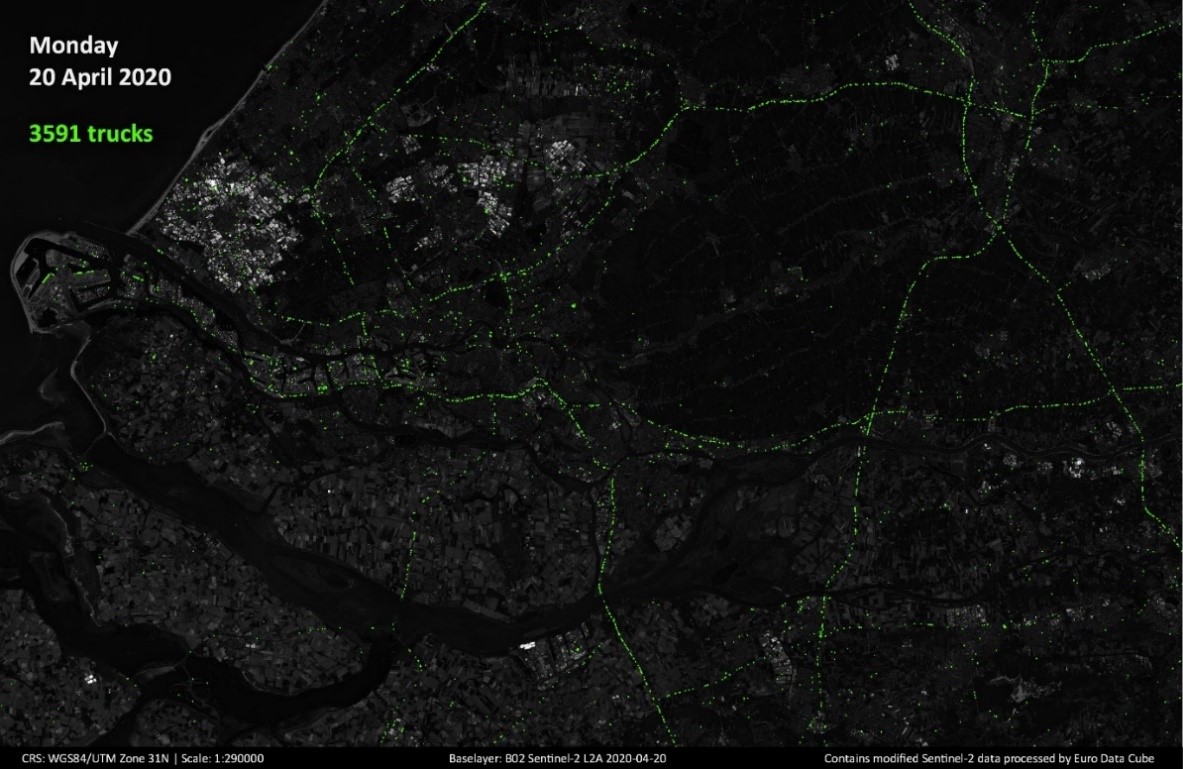
Source: hfisser github page

Rationale for choice of locations

We developed our method using two locations for predicting truck counts:

• a stretch of the M1 motorway between Leicester and Sheffield
• part of the main road running from Mombasa to Nairobi in Kenya

The M1 was chosen due to availability of reliable road sensor network data from Highways England to validate predictions. These data are disaggregated into vehicle size classes, so any vehicles under 5.2m were considered unlikely to be a commercial truck. Kenya was chosen due to our existing relationships with the Kenya National Bureau of Statistics and Trademark East Africa. Other advantages of the chosen location in Kenya were the availability of vehicle weighbridge data for ground-truthing and the road’s position near the port of Mombasa, a major hub of trade into East Africa.

Sentinel 2 Data

We extracted open-source Sentinel 2 images for areas of interest for the full range of image dates available, which began in 2017 for the UK and 2019 for Kenya. Images were extracted in three of the bands available from the Sentinel 2 surface reflectance collection;

• B2 (Blue)
• B3 (Green)
• B4 (Red)

These were chosen as they best distinguish trucks against the road – as a sequence of blue, green and red pixels against a grey/brown background. Additional bands for cloud probability and cloud shadow were extracted using the Sentinel 2cloudless algorithm from the Sentinel hub. The cloud probability band was used to mask out pixels above a threshold probability of 0.25 of being either cloud or cloud shadow. This threshold was chosen to balance the risk of more false positives generated by cloud edge at higher thresholds, and too much of the image being masked out at lower thresholds.

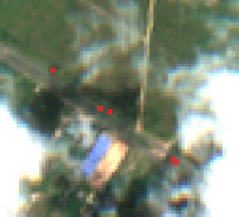
To explore features and validate the model predictions made with the Sentinel 2 images, we manually labelled the blue, green and red pixels of each truck in image for 10km stretches of road in the UK (the M1 motorway) and two locations outside of Nairobi, Kenya (Figure 2). These data have many more non-truck pixels than truck pixels. This class imbalance was an important consideration when designing our classification method, as it can bias our evaluation of model performance.

Figure 2: Example of a labelled truck in the red, green and blue bands in Nairobi, Kenya

Feature engineering

Our initial approach used an unsupervised classification algorithm directly in Google Earth Engine. This method uses hard-coded thresholds for hue, saturation, and brightness to automatically cluster images into truck or road pixels without prior labelling by eye. This generated predictions for whole countries very quickly, however it resulted in many false positives in cloudy images, due to the refraction of light at the edge of clouds producing a rainbow effect which was being misidentified as a truck (Figure 3).

Figure 3. False Positives generated by rainbow effect at the edge of cloud

To develop an understanding of the truck effect, we engineered a set of features in the spatial and temporal dimensions to use in a supervised learning pipeline. The absolute colour of the truck pixels changes across time and space due to variability in weather, seasonality and terrain. For this reason we used the relative colour values (i.e. the ratio of red to green rather than red value) to distinguish truck pixels from road pixels. Exploratory analysis of labelled truck pixels confirmed that the derived colour ratio bands showed stronger signals both across the time series in the pixel locations where trucks were present. For example, the red truck pixels show a stronger peak in the red to green band than the red band (Figure 4a). The colour ratio bands also showed a stronger signal between truck and non-truck pixels within specific imaging dates (Figure 4b).

Figure 4. Temporal and spatial signals of a red truck pixel from M1 training data

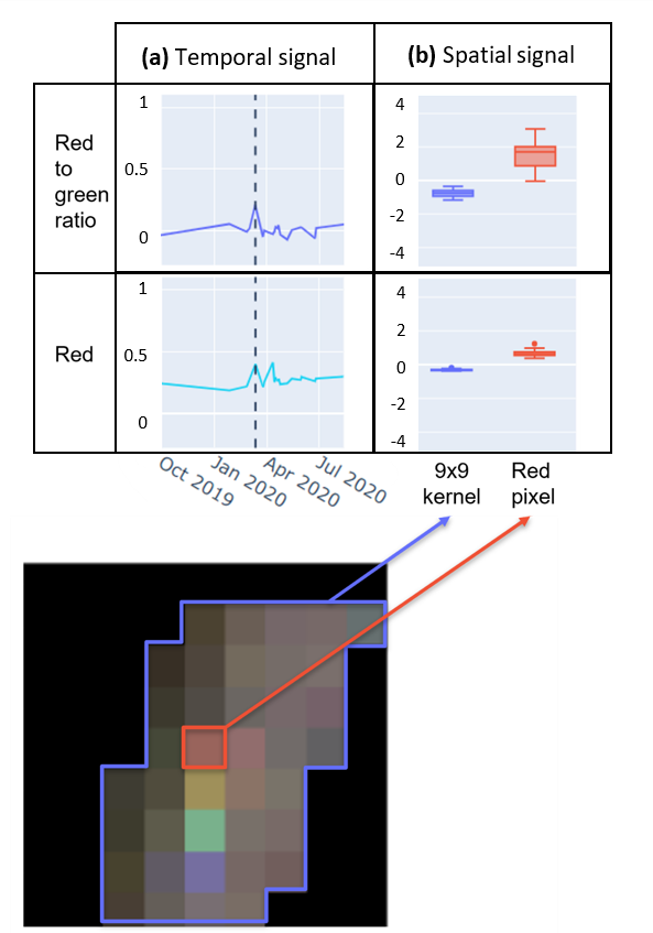
1. Time series of pixel values for colour and colour ratio bands (red:green = rg_img/rg) in the location where a truck was labelled.
2. The date where the truck was present is shown with a dashed line (a).
3. The pixel value of labelled truck and the mean value of pixels within a 9×9 kernel surrounding the red truck pixel in the red and red to green ratio bands (b)

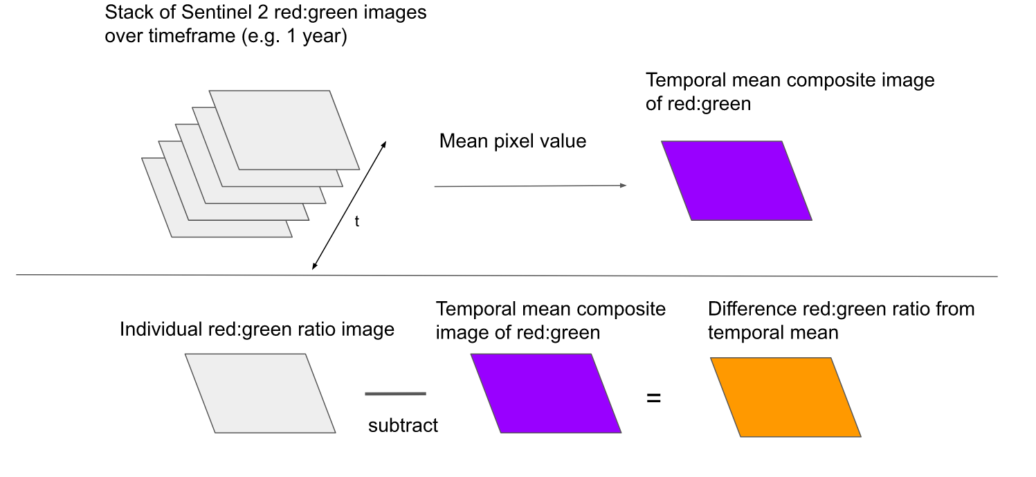
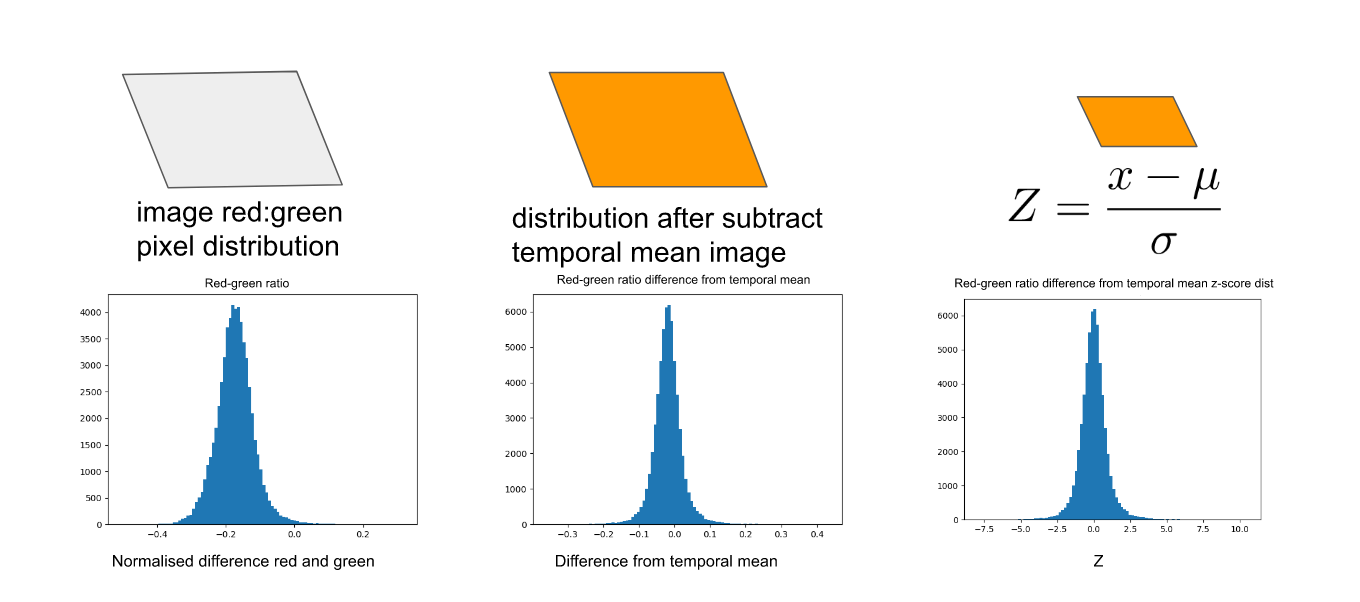
To improve the ability of our model to distinguish truck from non-truck pixels, we wanted a feature to capture the colour of a truck pixel relative to the mean colour over all dates in that pixel location. This is because each pixel corresponds to the same location across images and for any pixel location it is very unlikely that more than one imaging date will have a truck present. To detect this temporal signal, we created a composite mean image from all rasters in the time series and subtracted the temporal mean values for each feature from the feature values in a specific date, giving a ‘subtracted’ image. Finally, we calculated a Z-score for each pixel within this subtracted image:

\(\) \( Z = \frac { x \, – \, µ }{ σ }\)

Where x is the pixel value in the subtracted image, µ is the mean value across all pixels in the subtracted image and σ is the standard deviation across the subtracted image. Some images can be brighter or darker so without the Z score, all pixels in an image at a given date could be much higher or lower than the temporal mean and this would not be a useful measure to highlight the trucks (Figure 5).

Figure 5: Processing steps for temporal truck features

A crucial property of the truck effect is that the blue, green and red pixels are connected within a limited kernel space of a few pixels, so we created a feature which extended a small kernel from each pixel and recorded the most green and the most red pixels. We then elaborated on this to look for max R:G and G:R Z-scores, thereby capturing the temporal and spatial dimensions of the signal. This works by expanding a kernel of a few pixels outwards from each pixel in the G:R Z-score band (Figure 6.1), finding the local maxima (Figure 6.2), creating a mask from a small kernel surrounding the max G:R Z-score pixel (Figure 6.3) and using this to mask the R:G layer and find the max R:G value from the unmasked pixels (Figure 6.4).

Figure 6: Processing steps for developing neighboring pixel features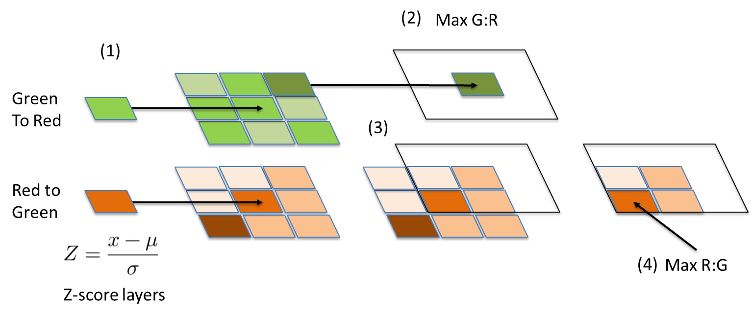

Modelling

We then derived these features in the labelled training data to train random forest classifiers from the python scikit learn package. We chose random forest classifiers as they produced higher F1 scores than logistic regression and support vector machines. We assessed model performance in predicting trucks from unseen dates by running a temporal cross validation; in each iteration of the train-test split, a different set of dates from the full series was used to train the model. We compared results using different origin of training data, old or old and new features included and either a low (1:10,000) or high (1:10) ratio of truck to non-truck pixels included in training data. Under sampling the majority class in imbalanced data can improve predictive performance of the minority class. To fit the model we would use on our new area of interest, a 100km stretch of road outside of Mombasa, model performance was measured on predictions for a combined training set of both locations in Nairobi with precision-recall area under the curve scores (PR AUC) calculated using stratified K-fold cross validation to ensure the class ratio was kept the same across folds. PR AUC visualises the trade-off between precision and recall for different probability thresholds of classification. PR AUC scores are advised over ROC AUC scores when using highly imbalanced data. After model predictions, we further calculated counts which were corrected by % cloud, so images with more cloud cover had boosted counts to compensate for lost image area:

\(Cloud \, weighted \, count = {predicted \, count} \left( \frac {100}{ 100 \, – \, percentage \, cloud }\right)\)

To scale up the process, we modified the pipeline to split each image into small tiles, which allowed feature generation and modelling to be run in parallel, allowing us to make predictions for 100km stretches of road within a few hours.

Challenges introduced by our methodology

Although the Sentinel 2 mission takes images at each location at frequent (five to ten day) intervals, in many countries the roads are obscured by cloud on many days in the year. This limits the number of images on which models can be trained and tested. The low resolution of the images (roughly 10 metres per pixel) means the truck effect can be hard to distinguish. Light refraction at cloud edge produces a rainbow effect which can be misidentified as a truck. To address the issue of false positives generated by cloud edge, we coded a 100 metre buffer around the cloud pixels in the cloud masking process. For all dates in Mombasa, this reduced the Pearson’s r correlation between % cloud pixels and truck probability from 0.63 to 0.005, and between % cloud pixels and cloud-weighted count from 0.33 to -0.04.

The Sentinel 2 2A product was only available as an operational product in Kenya from the end of 2018. The weighbridge data for the same location were also limited due to intermittent failure of the automatic sensor leaving few dates with intersecting satellite images and weighbridge counts to compare (n=30 dates with intersecting Sentinel 2 and weighbridge data).

Results and comparisons with external data

Including our newly engineered features improved model performance in the two manually labelled locations in Nairobi but did not improve performance for the labelled M1 location (Table 1).

Table 1. Results from temporal cross validation of random forest classifiers

Location	Features included	Class ratio	Number of training points	Precision	Recall	F1 score
M1	Extra derived features	1:10,000	323	0.65	0.41	0.50
M1	Extra derived features	1:10	323	0.41	0.84	0.55
M1	Basic features	1:10,000	323	0.67	0.41	0.51
M1	Basic features	1:10	323	0.41	0.82	0.54
Nairobi	Extra derived features	1:10,000	912	0.74	0.29	0.42
Nairobi	Extra derived features	1:10	912	0.19	0.82	0.31
Nairobi	Basic features	1:10,000	912	0.53	0.19	0.28
Nairobi	Basic features	1:10	912	0.15	0.80	0.25
Nairobi 2	Extra derived features	1:10,000	108	0.71	0.38	0.50
Nairobi 2	Extra derived features	1:10	108	0.25	0.71	0.37
Nairobi 2	Basic features	1:10,000	108	0.51	0.30	0.38
Nairobi 2	Basic features	1:10	108	0.21	0.78	0.33

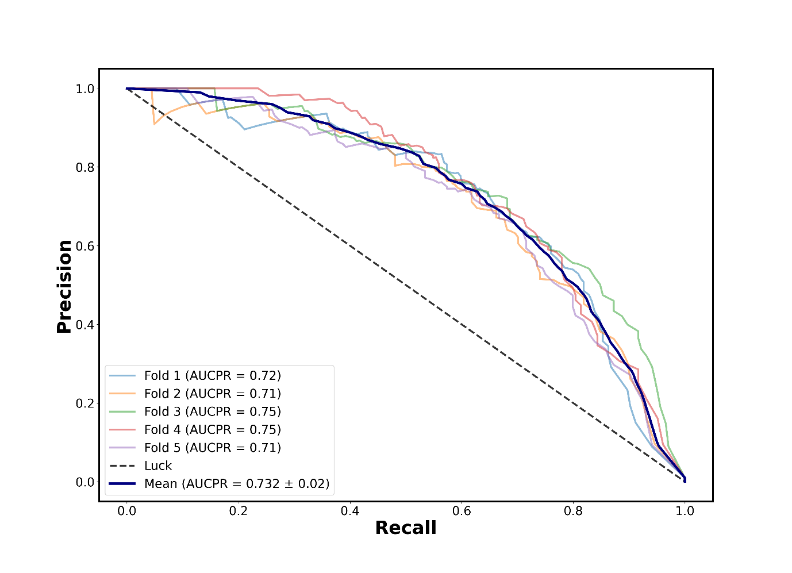
Stratified K-fold cross validation showed that models performed poorly when a low ratio of truck to non-truck pixels (1:10,000) was used (Figure 7a), but PR AUC scores improved substantially when the road pixels were more heavily down-sampled in the training set (Figure 7b).

Figure 7: Precision-recall curve from stratified k-means cross validation using labelled data from two locations outside of Nairobi, using a class sampling ratio of truck to non-truck of 1:10,000 (a) and 1:10 (b)

Figure 7a

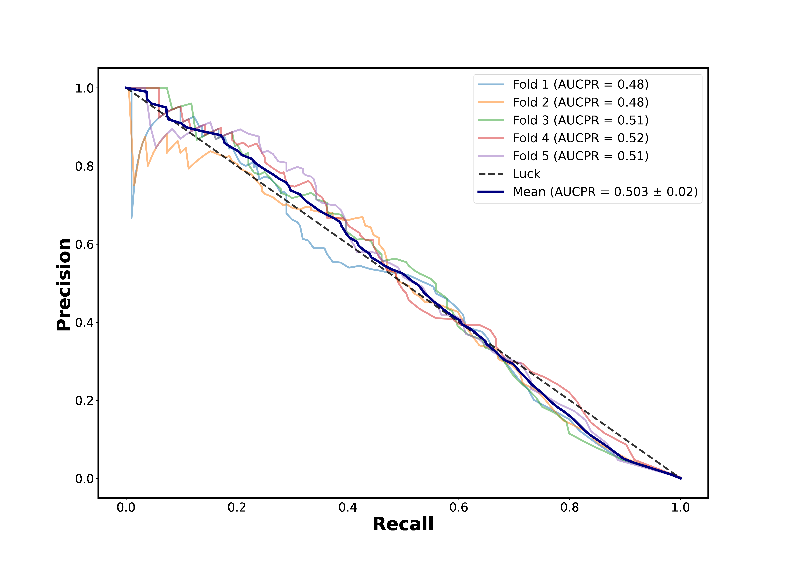
Figure 7b

However, when using this model to make new predictions on the longer 100km section of the same road from Mombasa, visual inspection of shapefiles indicated that a more heavily down-sampled model produced more false positives than models fitted to less balanced training data (Figure 8). This suggested heavily down-sampling was leading to overfitting.

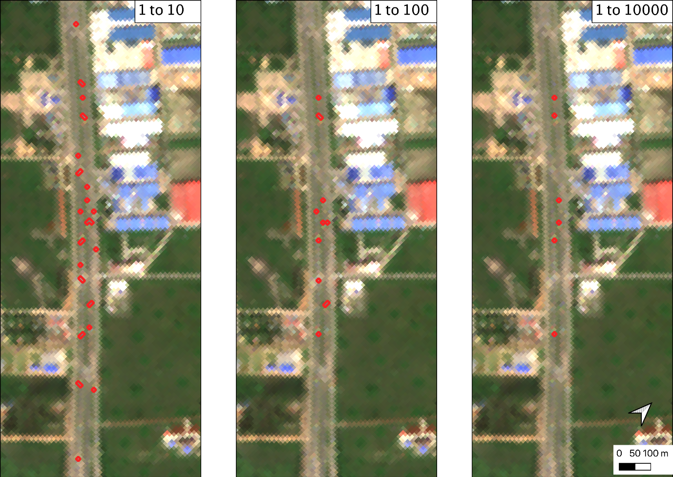
Figure 8: Mapping model predictions showed the most heavily down-sampled models (1:10 and1:100 truck to non-truck ratio generates many more false hits than the 1:1000 model)

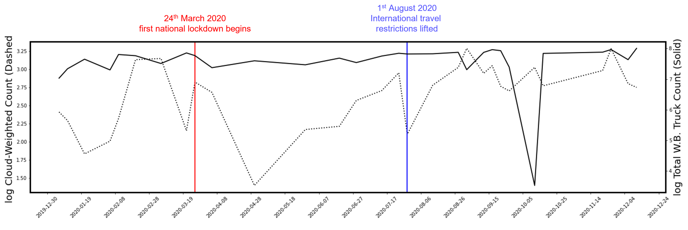
We tested how informative our predictions were by exploring whether we could see the expected drop in truck activity due to COVID-19 lockdowns. For a 100km stretch of the M1 motorway in the UK, we see a sustained drop in truck counts following the first national lockdown on 26 March, until the easing of restrictions is announced on 23 June. From this point, truck counts steadily increase until the announcement of Tier 4 restrictions around Christmas, followed by another sharp drop when the third national lockdown is announced (Figure 9).

Figure 9: Dates of lockdowns and restriction easings coinciding with drops and rise in predicted cloud-weighted truck counts (dashed line) and ground-ruth counts (solid lines) in 100km stretches of motorway on the M1 between Leicester and Sheffield (a) and outside of Mombasa, Kenya (b)

Figure 9a

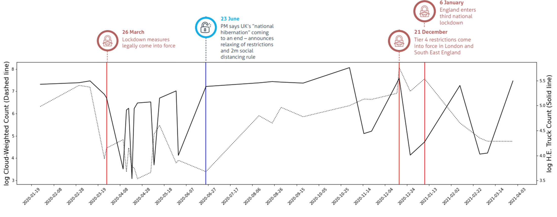
Figure 9b

We then compared our predictions to established data for vehicle traffic from automatic sensors. For the M1, Highways England data were given for different classes of vehicle size. From 2020 to April 2021, the strongest correlation was with the smallest vehicle class (Table 2a), suggesting our method was performing best with smaller commercial vehicles on the M1, as shown in Figure 10a, and smaller trucks in Kenya as shown in Figure 10b. This is probably because the volume of the more numerous small vehicles was more heavily affected by lockdowns and restriction easing than commercial trucks, so there is greater signal in the change of small vehicles than large trucks over the pandemic, despite smaller vehicles being individually harder to detect. On the M1, predictions are highly correlated with predicted counts (Spearman’s r=0.66) and cloud-weighted counts (Spearman’s r=0.88), suggesting unresolved issues with cloud and cloud shadow generating false positive.

Figure 10: M1 Highways England counts of vehicles under 0-5.2m and over 0-5.2m in length compared with Sentinel 2 based vehicle counts (a), truck Weighbridge counts from Kenya Highways Authority for smallest vehicle class and summed class counts compared with Sentinel 2 cloud-weighted counts (b), variables are log-transformed

Figure 10a

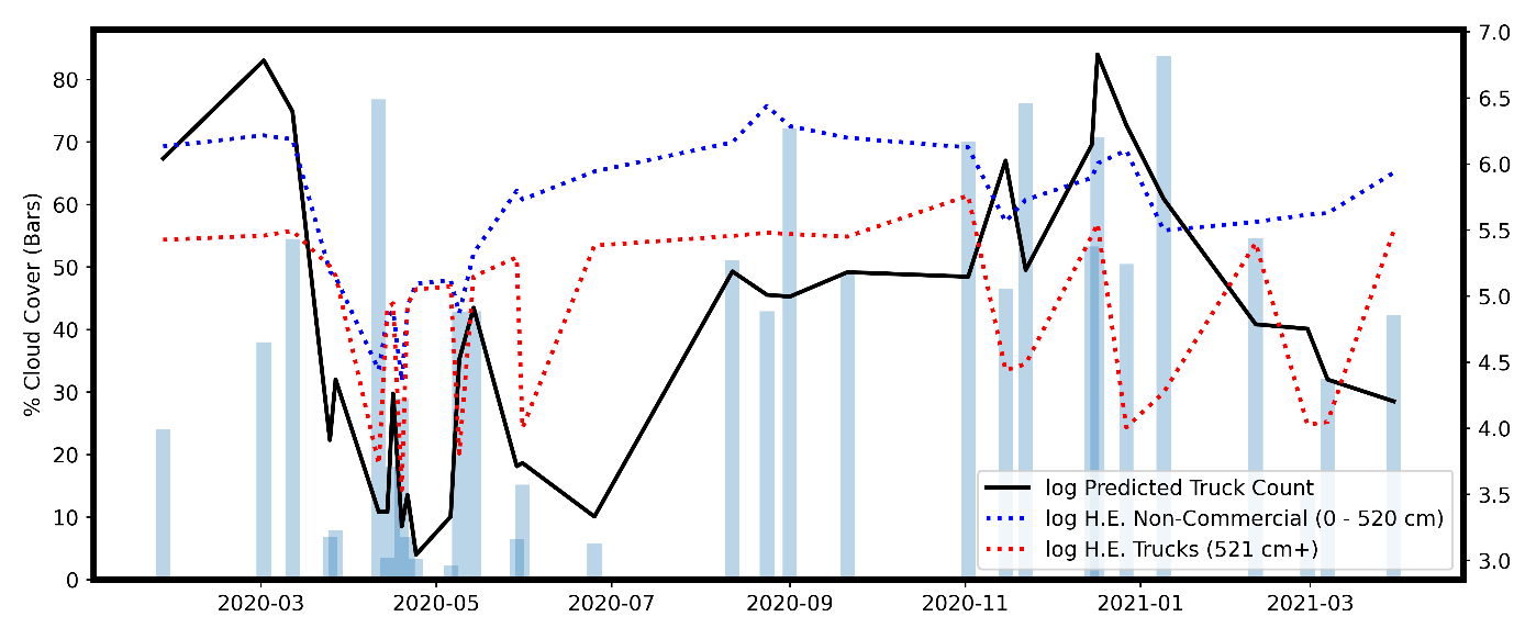
Figure 10b

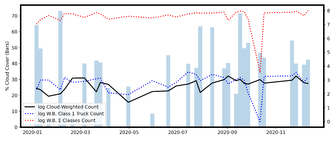
Table 2a. Spearman’s correlation coefficients between the M1 truck predictions, percentage of cloud pixels across image and the six vehicle class counts from Highways England

		% cloud	0 – 520 cm	1160+ cm	521 – 660 cm	661 – 1160 cm	Total Volume	Trucks (520+ cm)
Predicted Truck Count	P-value	0.00	0.00	0.03	0.01	0.03	0.00	0.02
	Spearmans r	0.66	0.65	0.38	0.45	0.38	0.60	0.42
Mean Truck Probability	P-value	0.00	0.53	0.22	0.40	0.17	0.38	0.31
	Spearmans r	-0.77	-0.11	-0.22	-0.15	-0.25	-0.16	-0.18
Cloud-Weighted Count	P-value	0.00	0.00	0.09	0.04	0.08	0.00	0.05
	Spearmans r	0.81	0.58	0.31	0.37	0.31	0.52	0.35

Table 2b. Spearman’s correlation coefficients between the Mombasa truck predictions, percentage of cloud pixels across image and weighbridge counts for each truck size class from Kenya Highways Authority

	Predicted Truck Count		Mean Truck Probability		Cloud-Weighted Count
	P-value	Spearmans r	P-value	Spearmans r	P-value	Spearmans r
% cloud	0.00	-0.54	0.80	0.05	0.96	0.01
Class 1	0.36	0.17	0.62	-0.10	0.13	0.29
Class 2	0.43	-0.15	0.42	-0.15	0.79	0.05
Class 3	0.25	0.22	0.55	0.11	0.09	0.32
Class 4	0.41	0.16	0.06	0.35	0.14	0.27
Class 5	0.22	0.23	0.88	-0.03	0.62	0.09
Class 6	0.48	0.13	0.70	-0.07	0.58	0.11
Class 8	0.06	0.35	0.47	-0.14	0.06	0.34
Class 9	0.23	0.23	0.85	0.04	0.43	0.15
Class 10	0.52	-0.12	0.72	-0.07	0.96	0.01
Class 11	0.39	0.16	0.89	0.03	0.14	0.27
Class 12	0.49	0.13	0.36	0.17	0.29	0.20
Class 13	0.68	-0.08	0.40	-0.16	0.56	-0.11
All Classes	0.43	0.15	0.73	0.07	0.13	0.28

Conclusion and next steps

Our preliminary work showed how Sentinel 2 imagery can be used with feature engineering and supervised learning methods to estimate traffic volumes on roads. Although our method was able to detect large changes to road traffic, such as the impact of lockdowns and easing of restrictions since the Covid-19 pandemic started, these methods are not robust enough to provide closer-to-real-time estimates as an alternative to traditional, sensor-based methods for road traffic estimation. We can attribute the low correspondence to scarcity in the ground-truth data for Mombasa, gaps in imaging due to cloud cover, correlation of M1 predictions with cloud and cloud shadow and ambiguity in the truck-effect. Access to ground truth data with better coverage and quality in developing countries, and improvements to the cloud shadow masking process are required to go forward with this project.

While our method did not provide a clear solution for the intended use-case, processes developed in geospatial processing and classification of open-source sentinel 2 data could be used in a range of future data science projects and learning resources.

For example, we have adapted the model fitting and evaluation scripts into a short course on supervised machine learning for next year’s cohort of graduate data scientists at the Campus.

A key lesson learned from the project is that working with novel data sources and methods requires planning evaluation from the start. Ensuring maximum coverage and quality of ground truthing data and identifying pitfalls in these data early on will determine whether the utility of new methods can be demonstrated effectively.

Please get in contact with Ruben Douglas to discuss this project including any ideas for future applications.