Faster indicators of UK economic activity: shipping

The Independent Review of UK Economic Statistics (Bean, 2016) stated that “the longer a decision-maker has to wait for the statistics, the less useful are they likely to be”. Faster UK economic indicators enable policymakers such as HM Treasury and the Monetary Policy Committee of the Bank of England to set appropriate policy more quickly in response to economic changes.
The Faster indicators of UK economic activity project, led by the Data Science Campus at the Office for National Statistics is a response to this challenge. The goals are to:
- identify close-to-real-time big data or administrative data sources which represent useful economic concepts
- create a set of indicators which allow early identification of large economic changes
- provide insight into economic activity, at a level of timeliness and granularity not possible for official economic statistics.
In this project, we have initially explored 3 datasets: HMRC Value Added Tax (VAT) returns, ship tracking data from automated identification systems (AIS), and road traffic sensor data for England. This paper describes the data, methodology and economic analysis for the shipping indicators. Information on the other indicators describing the time series up until the end of December 2018, and the full dataset, can be found in the following publications:
- Faster indicators of UK economic activity: summary
- Faster indicators of UK economic activity: Value Added Tax returns
- Faster indicators of UK economic activity: road traffic in England
- Faster indicators of UK economic activity: dataset (xlsx, 469kb)
It is important to note that we are not attempting to forecast or anticipate official gross domestic product (GDP) estimates or other headline economic statistics here, and the indicators should not be interpreted in this way. Rather, we provide an early picture of specific economic activity – in this case, shipping activity, related to trade in goods – which may be of interest to policy makers. It may be that these indicators have the power to improve the performance of nowcasting or forecasting models, as components of these models, but we have not as yet tested this.
In this paper, we present an initial exploration of the use of ship movements around the UK. Two new monthly shipping indicators have been derived from Automatic Identification System (AIS) data, the international system for tracking ship movements.
- ‘Time-in-port’ is based on aggregate time spent by ships in 10 major UK ports.
- ‘Total traffic’ is based on the number of unique ships entering the 10 major UK ports.
These indicators are likely to be important in supplementing our understanding of international trade activity. They offer a fast indication of the level of shipping activity, which is, as we show, related to trade in goods, by individual port. We compare data for July 2016 to August 2018 to official statistics for gross value added (GVA) and trade statistics. We find a surprisingly good correlation between the shipping indicators and imports, particularly given the noisy nature of these variables. However, care must be taken in the interpretation. We do not have a sufficiently long time series to be able to seasonally adjust it, so correlations may be driven largely by seasonal variation. Furthermore, although the overall correlation is reasonably good, individual points can deviate strongly. For these reasons, we do not recommend using these indicators on their own as predictors of GDP or other headline economic statistics.
The relationships between time in port and international trade in goods could potentially be used in a mathematical model in combination with other indicators to estimate trends in trade. Given the fact that AIS can be obtained in timely fashion, in fact in near real time, the output of such a model can be a valuable tool for early economic trend discovery.
Initially, we anticipate publishing monthly indicators with a one-month lag (i.e. publishing indicators for March in April). This is one month in advance of official estimates of GDP. The first publication is planned for mid-April 2019, with an article setting out the full set of faster indicators of UK economic activity (covering those based on VAT returns, road traffic data and shipping) and the format of the publication to be released in advance. Proposed future work includes the development of interactive visualisations to allow analysts and policy-makers to easily explore these new datasets in rich detail.
Section 1 discusses the data and its quality. The methodology is presented in Section 2, and the economic analysis in Section 3. We summarise our conclusions in Section 4, and discuss the potential for future work in Section 5.
We welcome feedback on this work, which can be sent to Faster.Indicators@ons.gov.uk
1. Data and data quality
The Automatic Identification System
The International Maritime Organization’s International Convention for the Safety of Life at Sea requires Automatic Identification System (AIS) to be fitted aboard international voyaging ships with 300 gross tonnage (GT) or more, and all passenger ships regardless of size. In practice, many more than the required ships have the equipment installed. AIS is used on ships to avoid collisions at sea, and by marine traffic authorities and analysts to monitor the movements of the vessels across the globe. By using satellite AIS data, a significant part of cargo ship movements around the globe can be captured.
Ships equipped with AIS equipment on-board transmit positional information every 2 seconds when moving and up to 3 minutes when anchored or moored. Originally introduced for navigational safety, AIS data can also be used as a source of information for monitoring trends in shipping activity.
Although there is inherent noise present in the signal, the position update frequency allows an improved precision for tracking ship locations and movements to be achieved by using Kalman filtering. The higher accuracy is a result of estimation of a joint probability distribution over the positional parameters for each timeframe. Overall, the less noisy estimated positions enable increased fidelity in identifying events such as entering and leaving port or estimating the docking positions. Also, because there is only a small delay in receiving AIS messages in a live stream, any derived outputs, like the proposed indicators, can be produced and published in a timely fashion. However, the timely processing of such large amount of information, approximately 28 million messages per day, requires substantial computational resources and suitable Big Data technologies. In this project, Apache Spark and a Hadoop cluster are used to manage the volume and velocity of the incoming AIS data.
In this work, we analyse 2 years of AIS data, from July 2016 to August 2018, for UK ports from the Maritime and Coastguard Agency. We also currently have access to real-time data from ORBCOMM, via the United Nations Global Platform, which can be used for future updates.
Data quality
Although the AIS dataset is clearly a large, rich source of data, some quality issues must be considered. For example, the ship crew can switch off the AIS equipment for various reasons, a state known in industry as “going dark”. The lack of signal from the ship results in a gap in the dataset for the duration of the event. If it represents a significantly long period it is possible that the ship port visit is only partially detected or not detected at all by the algorithm and the accuracy of the output is reduced. Fortunately, our exploration of the data in UK ports suggests that these events do not occur often and for the purpose of this work their impact on the outputs can be ignored. Additionally, some of the route information transmitted by the ship through AIS must be entered manually by the crew members. This includes useful information such as destination and previous/next port of call. However, the manual entries are not always completed on time, and may not always be accurate even when they are entered. For example, final route destination is reported for only 41% of journeys. To avoid any potential bias in the outputs which might arise from quality issues associated with the manual entry of data, this work has focussed on developing methods relying only on the data which is generated automatically.
In the project so far, we have not been able to identify the ship type, and the dataset includes passenger ships, pleasure craft, tug boats, fishing boats etc., as well as freight carriers. Potential future work may include exploring the availability of additional data sources which allow us to differentiate between different ship types.
Data preparation
The AIS messages are transmitted and stored in format specified by NMEA 0183 and IEC 61162-1 standards. There are twenty-four message types defined together with the structure of the information within each message type. For this work, messages of types 1, 2 and 3 are of most interest to us. They contain the automatic position report from the ship transponder. Table 1 lists in bold the variables used in this work and their position in the message structure.
Table 1: variables available in the AIS message types used in this work (bold), and their position in the message
| Position in message | Variable |
| 1-6 | Message Type |
| 7-8 | Repeat Indicator |
| 9-38 | Maritime Mobile Service Identity (MMSI) |
| 39-42 | Navigation Status |
| 43-50 | Rate of Turn (ROT) |
| 51-60 | Speed Over Ground (SOG) |
| 61-61 | Position Accuracy |
| 62-89 | Longitude |
| 90-116 | Latitude |
| 117-128 | Course Over Ground (COG) |
| 129-137 | True Heading (HDG) |
| 138-143 | Time Stamp (UTC Seconds) |
After removing of the duplicated and corrupted messages and subsequent decoding, the time stamp, latitude and longitude variables are extracted from the raw AIS data to compute the aggregate outputs as described in Section 2.
More information about AIS data, and its use in analysing ship behaviour in ports can be found in the article ‘Analysing port and shipping operations using big data’ (Bonham et al., 2018).
2. Indicator methodology
Data cleaning
In order to reduce the noise in the dataset, all the AIS messages from ships that have reported positions within a small area over the two-year period have been removed. The area size is a selectable parameter in the algorithm, currently set to 30 miles. This measure has removed all one-off erroneous messages. As the threshold is significantly high, it has also removed the data sent by the ships that do not leave port and therefore are considered not to contribute directly to trade.
Port definitions
The UK ten biggest ports by cargo in 2017 as reported by the Department for Transport in ‘Port freight annual statistics: 2017 final figures’ are listed in Table 2, together with the latitude and longitude and a map illustration of the rectangular bounding boxes defining the port boundaries. These areas were manually defined from a map for each port using the typical berth positions. In the case of Grimsby & Immingham, due to the distance between the sites, two bounding boxes have been defined and the presence of a ship in either of them is considered in-port state. These ten ports cover around 70% of total UK port freight (2017).
Table 2: the UK’s ten biggest ports by cargo (2017), the latitude and longitude for the rectangular bounding boxes defining the port boundaries in this work and their map illustrations
| Port Name | Bounding box: top left corner / (latitude, longitude) | Bounding box: bottom right corner / (latitude, longitude) | Map |
| 1. Grimsby
& |
( 53.5841 , -0.092023 )
|
( 53.572616 , -0.055467 )
|
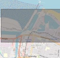 |
| Immingham | ( 53.6505 , -0.2183 ) | ( 53.6189 , -0.1548 ) |  |
| 2. London | ( 51.5262 , -0.1203 ) | ( 51.4415 , 0.5869 ) |  |
| 3. Southampton | ( 50.9123 , -1.4898 ) | ( 50.8761 , -1.3532 ) |  |
| 4. Liverpool | ( 53.4630 , -3.0544 ) | ( 53.3850 , -2.9751 ) |  |
| 5. Milford Haven | ( 51.7134 , -5.1313 ) | ( 51.6862 , -4.9274 ) | 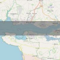 |
| 6. Felixstowe | ( 51.9682 , 1.2511 ) | ( 51.9308 , 1.3280 ) | 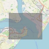 |
| 7. Tees & Hartlepool | ( 54.7109 , -1.3076 ) | ( 54.5663 , -1.1003 ) | 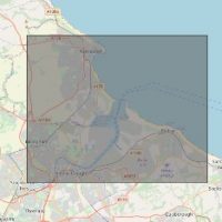 |
| 8. Forth | ( 56.1454 , -3.8249 ) | ( 55.9468 , -2.9391 ) | 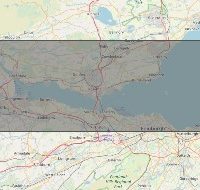 |
| 9. Dover | ( 51.1333 , 1.2978 ) | ( 51.1052 , 1.3548 ) | 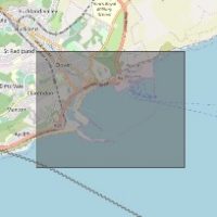 |
| 10. Belfast | ( 54.6432 , -5.9227 ) | ( 54.6025 , -5.8725 ) |  |
A ship is considered in port for the period until the next message arrives if its reported position is inside the port bounding box. The in-port states are marked from 1 to 10, corresponding to the port number listed in Table 2. If the ship position does not fall in any of the defined port bounding boxes then the in-port state is left in its default value, 0, defining a group of ships that are out of port. The in-port state is used to group the data and compute the aggregations per port as described below.
Aggregation
The data is then grouped by the in-port state of the ship to produce the outputs for each of the ten ports individually, and then aggregated for all ports. The ‘time-in-port’ indicator is computed by summing all the periods of the time spent of ships having in-port state corresponding to the port over each port and each month. In cases when a ship’s AIS transponder is switched off inside a port the time of its contribution to the indicator is considered only if the following message received from the ship is also within the same port. This rule eliminates the outliers in data resulting from moored ships switching off their AIS equipment and later leaving port without reactivating it or from ships that for some reason change their Maritime Mobile Service Identity (MMSI) while in port.
Similarly, the ‘total traffic’ indicator is computed by grouping the data by month and by in-port state and counting the number of unique ships, identified by their MMSI numbers. In cases when there two or more different reported positions in the very short period of time, perhaps due to noise, if one of these positions is within the defined port area the ship presence is counted in the indicators.
As the total traffic indicator measures the number of unique ships entering port each month it is not sensitive to ships that spend very long periods in port, e.g. pilot boats, or to have frequent port calls, e.g. ferries. On the other hand, the ‘time-in-port’ captures all time that ships spend in port and it may increase relative to the ‘total traffic’ indicator if either there are delays in port, or it takes longer to upload ships due to more cargo on board.
3. Economic analysis
In this section, we analyse the relationship between the two shipping indicators and official economic statistics. As we have only two years of data for the shipping indicators (July 2016 – August 2018), this analysis is necessarily limited, and we cannot see how our new indicators behaved during a recession. Also, because we have less than 3 years data, we are not able to seasonally adjust the shipping indicators at present. As we construct a longer time series, we will explore the impact of seasonal adjustment on the relationship between shipping indicators and official economic statistics. However, it is useful to explore these relationships as far as is possible, particularly as it might help identify future areas of research. We also remind the reader that the primary goal of this work is the early identification of unusual port activity and whether there are any early steers in that information, not to predict official economic statistics.
The economic statistics we compare our new indicators with are those which are available on a monthly basis, and which are likely to be relevant for the shipping indicators. They are:
- monthly gross value added (GVA), chained volume measure, seasonally adjusted (CVM, SA), source: Office for National Statistics (ONS).
- monthly trade in goods, imports and exports, current prices (CP), SA, source: ONS.
- monthly UK overseas trade statistics, imports and exports, CP, NSA, source: HM Revenue and Customs (HMRC).
GVA
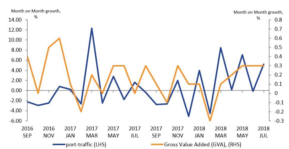
Figure 1 presents a comparison of the month-on-month growth rate for time-in-ports with GVA. The Pearson correlation coefficient for the series is 0.23, a weak, positive relationship. Figure 2 shows a comparison between the month-on-month growth of the total port traffic indicator and month-on-month growth of GVA. Total port traffic also has a weak, positive relationship with GVA, with a correlation coefficient of 0.26. Trade in goods is only one component of GVA, and is defined by change in international ownership in this National Accounts estimate, rather than transfer across international borders, which one might expect the indicators based on shipping activity to better reflect. However, it is reassuring that there is still a positive correlation with GVA, even if it is, as might be expected, weak. Seasonal adjustment of the shipping indicators, were it possible, might improve this relationship.
The UK is one of the more open advanced economies, with the sum of its real export and import flows being equivalent to around 60% of UK real GDP. This highlights the potential value there is in being able to explore whether there is a signal in these early shipping indicators, as developments in the global economy can transmit to the UK through such trading channels. It is possible that this will also capture other channels through which shocks might affect the UK economy. For example, if the recent uncertainty that appears to have weighed upon capital investment by businesses through 2018 might be showing upon how able and willing firms are to engage in international trade. Alternatively, business surveys point to there being increased evidence of stockpiling taking place as part of preparations ahead of the UK’s planned departure from the European Union, so it might be that these shipping indicators might capture increases in imported final and intermediate goods.
Figure 1: month-on-month growth rates for the time-in-port indicator and GVA (CVM, SA). Source: ONS
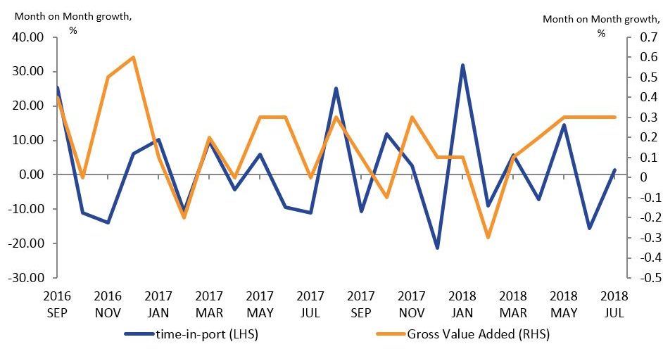
Figure 2: month-on-month growth rates for port traffic and GVA (CVM, SA). Source: ONS
Imports
Figures 3 and 4 show the relationship between growth in imports of goods (as estimated by both ONS and HMRC) and time-in port and total port traffic respectively. For the HMRC overseas trade estimate, international trade is defined as the movement of goods across international borders. For the ONS estimates, produced in accordance with the European System of Accounts 2010 (ESA2010), trade in goods is defined as a change in international ownership. One might expect, therefore, that shipping would correlate better with HMRC estimates than the ESA2010 definition, however, both estimates show a reasonable correlation with both shipping indicators. For time-in-port, the correlation coefficients are 0.45 (HMRC) and 0.43 (ONS). For total port traffic, they are 0.56 (HMRC) and 0.64 (ONS).
For example, differences between the official statistics and the shipping indicators will also arise because:
- at present, we include all ship types, not just cargo ships
- not all imports to the UK come via the sea
- we do not have information on the value (or type) of goods being transported
- some shipping will be between UK ports, rather than international voyages.
Figure 3: month-on-month growth rates for the time-in-port indicator and imports of goods (CP). The ONS estimates have been seasonally adjusted. Source: ONS, HMRC
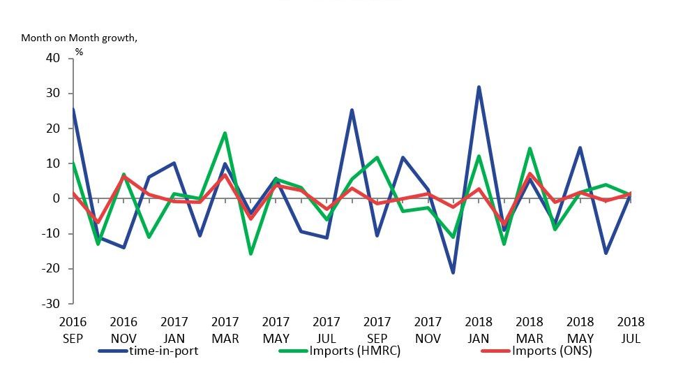
Figure 4: month-on-month growth rates for port traffic and imports of goods (CP). The ONS estimates have been seasonally adjusted. Source: ONS, HMRC

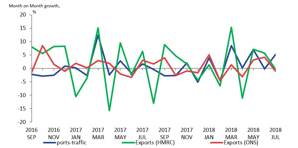
Exports
Figure 5 shows a comparison between export growth rates and the growth rate of the time-in-port indicator, and Figure 6 shows the export growth rates with the total port traffic indicator. Exports for both the ONS and HMRC estimates are shown.
The correlation between exports growth and growth of the time-in-port indicator is negligible at 0.06 (HMRC) and 0.07 (ONS). For port traffic, the correlation coefficients are much better, 0.48 (HMRC exports) and 0.23 (ONS exports).
It is interesting that the shipping indicators correlate better with imports than exports, especially for the ONS statistics. This reason for this can be further explored when we have a sufficiently long times series to be able to carry out seasonal adjustment of the shipping indicators.
Figure 5: month-on-month growth rates for the time-in-port indicator and exports of goods (CP). The ONS estimates have been seasonally adjusted. Source: ONS, HMRC

Figure 6: month-on-month growth rates for port traffic and exports of goods (CP). The ONS estimates have been seasonally adjusted. Source: ONS, HMRC
4. Conclusions
We have compared shipping data for July 2016 to August 2018 to official statistics for gross value added (GVA) and trade statistics. Table 3 summarises the correlations between month-on-month growth rates for our shipping indicators and the economic statistics to which we have compared them. We find a surprisingly good correlation between the shipping indicators and international trade in goods, especially imports, particularly given the noisy nature of these variables. However, care must be taken in the interpretation, as can be seen in the scatter plot in Figure 7, which shows the relationship between time in port and the ONS estimate of imports. We do not have sufficiently long time series to be able to seasonally adjust the shipping indicators, so correlations (or the lack thereof) may be driven at least in part by seasonal variation. As we build a longer time series, this is something we can explore further. Furthermore, although the overall correlation is reasonably good, individual points can deviate strongly. For these reasons, we do not recommend using these indicators as predictors of GDP or other headline economic statistics on their own, although they do offer a fast indication of the level of shipping activity, which is, as we have shown, related to trade in goods, by individual port.
The full datasets, including breakdowns by port, can be found in Faster indicators of UK economic activity: dataset.
Table 3: correlation coefficients for the month-on-month growth rates for the shipping indicators and the economic statistics to which we have compared them
| GVA | Imports (HMRC) | Imports (ONS) | Exports (HMRC) | Exports (ONS) | |
| Time-in-Port | 0.23 | 0.45 | 0.43 | 0.07 | 0.06 |
| Port traffic | 0.26 | 0.56 | 0.64 | 0.48 | 0.23 |
Figure 7: scatter plot showing the relationship between port traffic growth rates (%) and the ONS estimates of imports of goods (%).
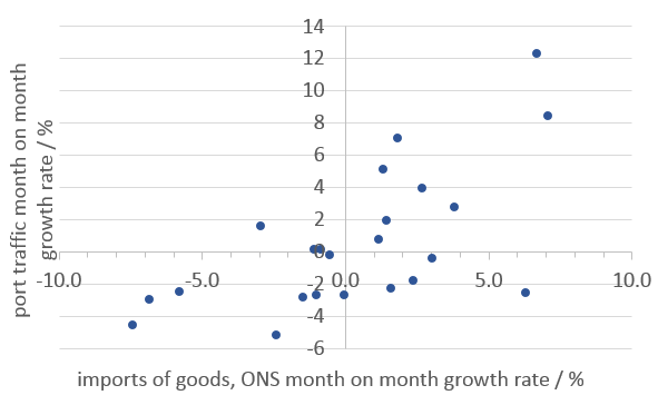
Although the period of two years, currently limited by our available AIS data, is not sufficient to draw robust conclusions about the links between the proposed shipping indicators and the official economic estimates, the relatively good correlation of 0.64 between port traffic and import of goods estimated by ONS suggest a relationship between the two measures. Such a relationship could be used by a mathematical model in combination with other indicators to estimate trends in trade. Given the fact that AIS can be obtained in timely fashion, in fact in near real time, the output of such a model can be a valuable tool for early economic trend discovery.
5. Further work
This work represents the first initial rapid exploration of these data, together with the first publication of the datasets. Further analysis and enhancements to the datasets are also proposed.
As a priority, we intend to publish regular monthly updates for these indicators, including indicators for each of the individual ports, from mid-April. These estimates will be published one month after the reference month (e.g. for indicators for March will be published in April), in advance of the official GDP estimates. The first publication is planned for mid-April 2019, with an article setting out the full set of faster indicators of UK economic activity (including those based on VAT returns and road traffic flow) and the format of the publication to be released in advance.
As the individual shipping ports have different import and export product profiles, it is our intention to study the links between the proposed time-in-port and port traffic indicators and port product profiles at the individual port level. The products can be linked to specific industries, allowing a deeper analysis of the relationship between shipping and the UK economy. Furthermore, the known cargo specialisation of certain berths, due to the installation of specific loading equipment, creates a unique opportunity to obtain sub-port versions of the indices and explore their links with sectors of economy.
It is natural to anticipate that the movements of bigger ships are more important to the economy than these of small leisure boats. Therefore, if suitable ship register data become available, it will be possible to produce disaggregated sub-indices, representing the motion patterns of different groups of ships. These will be investigated for links with different economic indicators. Subsequently, combining the sub-indices using different weights will enable the creation of weighted versions of the proposed indices that are expected to be more sensitive to detecting underlying economic trends.
We would also like to explore changing patterns of activity between ports. We could, for example, monitor changes in both the number and type of ships at each port, for both international and UK-to-UK journeys, if we have access to suitable ship register data.
The timeliness and coverage of the shipping indicators shown here have the potential to offer real-time insights into how the UK and global economy is evolving. The latest Economic Outlook by the Organisation for Economic Co-operation and Development (OECD) highlights a loss in global momentum and a sharp slowing in global trade, in part reflecting recent trade tensions. Expanding the study on a global scale is of significant interest as it might offer the possibilities of understanding how the global economy is evolving in close to real time, while it will allow investigation of network effects and studding of ship movement patterns between trade partners and how these may evolve over time.
Finally, we anticipate developing interactive visualisations of the shipping indices, to allow analysts and policy-makers to easily explore these new datasets in rich detail. We could potentially link this with our new road traffic data, to explore its use as an indicator of how quickly goods are moved around the country.
6. Authors
Alex Noyvirt, Ioannis Kaloskampis, Stephen Campbell, Sumit Dey-Chowdhury, Louisa Nolan