Data science for the public good

In this guest blog post, Federico Botta and Robin Lovelace talk about working as data science fellows with the data science team (10DS) at 10 Downing Street and the Office for National Statistics (ONS) Data Science Campus using transport data from the Department for Transport (DfT) to create Journey Time Statistics (JTS) R and Python packages. These packages import, process and visualise JTS data, eliminating the need for users to spend time cleaning the data and provide a reproducible pipeline for analysis.

---

Introduction

Making government data publicly available has a host of benefits. Public sector bodies that own and publish datasets can unlock value by opening anonymised datasets for use by a range of stakeholders, including enquiring citizens and journalists, academics and educators.

Open datasets can be used to better understand society, health, education, transport, the economy, and more. Open datasets are essential to evaluating policy in an open and reproducible way. Fully open data and analysis help to ensure data-driven research is democratically and scientifically accountable. The more people who are able to work on a dataset, the more likely we are to see these benefits unlocked.

So, it is important that data are not just publicly available, but that they are accessible, in a form that encourages reproducible data science. This blog post uses transport data as a case study to show how, when it comes to delivering the maximum public good, making data open is only part of the story, and that making it accessible matters.

The challenges of analysing open access data

Even when data sets are open, there can be barriers to analysing or comparing them. For example, the Department for Transport’s STAT19 datasets on road traffic casualties are all openly available but are hard to use because they are provided in untagged .csv files. The stats19 R package, which has been peer reviewed and published by the organisation rOpenSci, makes it easy for anyone to access the data in a reproducible format. This “packaging” of code enables researchers and others to focus on the research and policy impact rather than “reinventing the wheel” by spending time cleaning data.

The Department for Education (DfE) school places scorecards are also openly available, to provide another example. Comparing school ratings over time is still cumbersome because of differences in data formats and variables across different years. This can be challenging, particularly if you are trying to develop an analytical pipeline using a data science platform, which relies on a consistent data format.

Therefore, simply making datasets open is not always enough to ensure they will be used. Additional value can be unlocked by making data both openly available and easily accessible for analysis – a principle that applies especially to the kind of open data that governments provide.

To fully make use of open datasets in reproducible data science pipelines, data sets should be made available in analysis-ready formats that tools such as the R and Python programming languages can use. These languages dominate data science work in government, industry and academia.

Visualising JTS data with the jtstats packages

Our project demonstrates that data must be made accessible to maximise its impact and value. To this end, we use data on Journey Time Statistics (JTS), released by the Department for Transport, as an example of how further value can be added to open datasets by creating tools to easily analyse them.

We have developed R and Python packages that are able to import, process and visualise the JTS data. These packages eliminate any processing step needed by anyone interested in working with JTS data, thus reducing entry barriers to working with the data, as well as allowing for a reproducible pipeline based on our packages, rather than individually developed, ad-hoc scripts. This improves efficiency, reduces the risk of errors in the processing of the data, and overall helps to improve the quality of the analytical pipeline.

As an example, our packages allow easy retrieval and mapping of data on the average journey time to employment centres (with 100 to 499 jobs) by public transport simply by running the following lines of code.

In R:

install.packages(“remotes”)
remotes::install_github(“datasciencecampus/jtstats”)
library(jtstats)
jts_geo = get_jts(type = "jts04", purpose = "GPs", sheet = 2017, geo = TRUE)
names(jts_geo) # show the many columns available in the dataset

jts_geo |>
  select(GPPT15pct) |>  plot()

In Python:

import jtspy as jts

jts_df = jts.get_jts(type_code="jts05", spec="employment", sheet=2019, geo=True)
jts.choropleth_map(
    jts_df,
    "500EmpPTt",
    title="Travel time to jobs by public transport",
    cblabel="Average travel time in minutes",
    logscale=True,
    cbticks=[1, 10, 100],
    cbticklabels=["1", "10", "100"],
    linewidth=0.001,
)

Figure 1 shows a map of the United Kingdom displaying the percentage of people in different areas who can access a GP surgery within 15 minutes by public transport. The data are plotted at the Lower Layer Super Output Area (LSOA) and are plotted on a logarithmic scale for ease of visualisation. We can easily notice how urban areas, such as London and Manchester, have a much shorter travel time on average compared with rural areas, such as the North and South West of England.

Figure 1: A map of England showing the percentage of people in different areas who can access a GP surgery within 15 minutes by public transport.

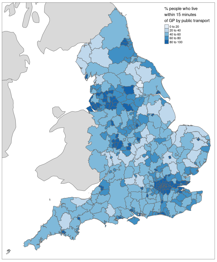
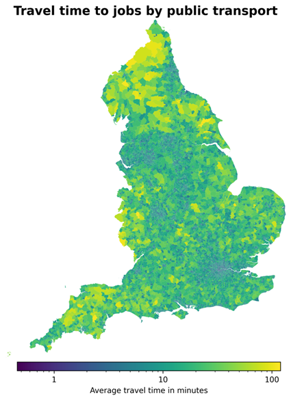
Figure 2 shows a map of the United Kingdom depicting how the average travel time to jobs by public transport varies in different LSOAs, plotted on a logarithmic scale. The map clearly illustrates the strong differences in accessibility to jobs between urban areas, such as London and Manchester, and rural areas, such as the South West and the North of England.

Figure 2: A map of the United Kingdom depicting the average travel time to jobs by public transport at the LSOA level. The values are plotted on a logarithmic scale to aid visualisation.

The JTS data are originally released by DfT in the open document spreadsheet (ods) format in a large number of different tables and files. Our packages rely on the version of those files that we converted to the more commonly used comma separated values (csv) format, which are then imported and processed by the R and Python code. The command-line script used to convert the files is also openly available on the JTSTATS repository.

While we believe our approach showcases the opportunities of developing these kinds of tools, there are always further improvements that could be implemented.

First, removing the conversion step from ods format to csv would further improve the reproducibility of our tools and minimise pre-processing steps. In fact, we suggest that, in the future, an alternative option could be to make data from public bodies available in more data science-friendly and memory-efficient formats, such as Apache’s Parquet format. However, it is also important to acknowledge that csv is a very widespread and popular format, which is unlikely to be replaced in the short term, so the development of reproducible tools based on csv files is going to remain relevant for most applications.

Second, in the case of tools developed across multiple programming languages, rigorous multi-language tests should be implemented to ensure that results obtained are consistent across the different languages.

Advancing open government data analysis

The approach presented here demonstrates the potential of coupling open government data with open reproducible data science tools, and we hope to encourage the adoption of such practices across all public bodies.

Building on our work, we advocate the creation of packages to support reproducible data science pipelines to allow a broader range of analysts, data scientists, and researchers, to use government datasets in their work. Such tools cannot only improve efficiency and reduce risks of errors in data processing, but crucially, can enable a broader audience to add value to public sector data.

Read a more detailed discussion of the jts package. The codes for jtstats, jtstats-R and jtstats-Py are available on GitHub.