Green spaces in residential gardens
A United Nations report showed that in 2014 approximately 54% of the population were living in towns and cities, with this figure projected to increase to 70% by the middle of the next century.
Identifying and understanding the features of urban green spaces (such as residential gardens) is therefore becoming of greater importance, given their environmental and emotional benefit.
Current approaches often assume residential gardens are almost exclusively covered by natural vegetation and do not take in to account urban areas such as steps, patios and paths.
We collaborated with Ordnance Survey (OS) to improve the current approach to identifying the proportion of vegetation for urban residential gardens in Great Britain. We used remote sensing and machine learning techniques with high-quality aerial and satellite imagery to test approaches. From the results, a tool able to classify the contents of an image with accuracy – a neural network classifier – was developed.
The initial results obtained using this approach estimate that 62% of garden space in Great Britain is vegetation. Data sampled from Cardiff and Bristol suggest that residential gardens in these areas contain approximately 54% and 45% vegetation respectively.
The methods and results presented in this report are from early research and are provided to assess the performance of the approaches tested. They are not official estimates and should not be interpreted in this way.
Table of contents
- Introduction
- Data
- Vegetation detection
- Unlabelled test image library
- Application to Bristol and Cardiff
- Labelled test image library
- Vegetation detection using infra-red spectral bands
- Vegetation detection using supervised machine learning
- Deployment
- Final Results
- Practical applications
- Summary
- Future work
- Acknowledgments
- Appendix: Application of the test algorithms to the unlabelled test image library
- References
1. Introduction
In 2014 approximately 54% of the population were living in towns and cities, this figure is projected to increase to 70% by the middle of the next century (United Nations, 2014). Consequently, urban green spaces such as residential gardens are of great environmental and emotional benefit to a population. A recent study has shown that access to green space has a positive impact upon mental health (White and others, 2013). Green spaces absorb more carbon than they return to the atmosphere (Nowak and others, 2002) and reduce air pollution (Nowak, and others, 2006). Impermeable materials that are increasingly used to replace green spaces such as garden paths or patios increase rain water runoff and the likelihood of flooding (Ellis, 2002). Residential gardens also act as wildlife corridors that help animals, birds and insects move between larger green areas supporting diversity and promoting the pollinator populations such as bees and butterflies (Rouquette, 2013 and Baldcock and others, 2015).
With this in mind, it is no surprise that measuring the proportion of vegetation in Great Britain’s residential gardens and tracking changes over time is a vital area of interest to the Office for National Statistics (ONS) and Ordnance Survey (OS). Ordnance Survey, Britain’s National Mapping Agency maintains Private Garden extents across Great Britain as part of its OS MasterMap suite of geospatial data assets. Although useful to define the extent of private gardens – when utilised as a green space or vegetation asset they often lead to an assumption of complete natural surface coverage. This contributes towards a key disadvantage in that it is almost always an overestimate of natural capital as residential gardens will have some urban areas (steps, patios, paths etc.). Ordnance Survey’s Geospatial Content Improvement Programme (GCIP) has the objective to capture or update physical features that reflects construction, demolition or other alterations in the real world. When revised and updated content is available these in-garden structures are accounted for within the private garden geometry. However, additional urban surfaces such as patios, decking and artificial turf remain fully encompassed in the polygon extent.
With the recent advent of readily available and high-quality aerial and satellite imagery much activity has focussed upon identifying features such as water, crops and soil erosion using remote sensing. This report details the work undertaken at the Data Science Campus in collaboration with Ordnance Survey (OS) to use remote sensing and machine learning techniques to improve upon the current approach used within the ONS to identify the proportion of green space for urban residential gardens in Great Britain.
Several “off the shelf” and bespoke techniques developed by both the Campus and OS are used to detect the presence of vegetation. They are assessed both qualitatively on a library of 10 representative gardens and quantitatively on 100 manually labelled gardens selected randomly from Cardiff and Bristol. The sensitivity of these algorithms to shadows within the imagery is discussed and techniques applied to reduce its impact. Finally, a neural network is trained on the manually labelled library, this network classifies areas within a residential garden to one of following categories:
- vegetation
- vegetation in shade
- urban in shade
Results are encouraging and suggest that the neural network can accurately classify areas of vegetation and is less susceptible to the effects of shadows when compared with the other test algorithms.
2. Data
The data used during this project is split into two groups
- garden parcel polygons
- aerial imagery
Garden parcel polygons
Private residential garden parcels have been derived through the geospatial analyses of multiple Ordnance Survey (OS) datasets licensed through the Public Sector Mapping Agreement (PSMA). This analyses involved using PSMA data to derive inferred property extents. These extents were used to collect and aggregate garden geometries together on a property-by-property basis within built-up-areas to form an indicative, functional garden extent. These extents do not define legal property ownership nor act as registered title extents. Datasets used included OS AddressBase Plus and OS MasterMap Topography Layer.
OS AddressBase Plus is a vector address point dataset for Great Britain that contains current properties and addresses sourced from local authorities identified using a Unique Property Reference Number (UPRN), matched to a series of third-party datasets including:
- Royal Mail’s Postcode Address File (PAF)
- Valuation Office Agency’s council tax and non-domestic rates
- OS large scale vector mapping
OS MasterMap Topography Layer is a vector dataset providing individual real-world topographic features in Great Britain represented by point, linestring, and polygon geometries, captured at 1:1250, 1:2500 and 1:10 000 scales in urban, rural and mountain or moorland areas respectively.
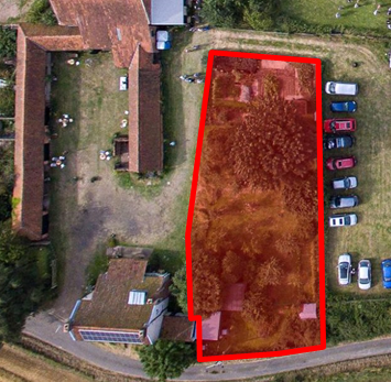
Figure 1: Polygon defining a garden boundary
Garden polygons for both Cardiff and Bristol were supplied in GeoJSON format, where each garden has a unique Topographic Identifier (TOID). The polygon was defined by a series of longitude and latitude co-ordinates as shown in Figure 1. 79,643 polygons were provided for Cardiff urban residential gardens and 209,205 were provided for Bristol.
Aerial Imagery
JPEG format aerial imagery was provided by Bluesky International Ltd and Getmapping Plc via the Public-Sector Mapping Agreement (PSMA). RGB images were provided at 12.5, 25 and 50 centimetre (cm) resolution and colour infra-red provided at 50 cm resolution. The geographical coverage of the images is shown in Figure 2.
Figure 2: Image coverage, colour scale represents time period from 2006 (red) to 2017 (blue)
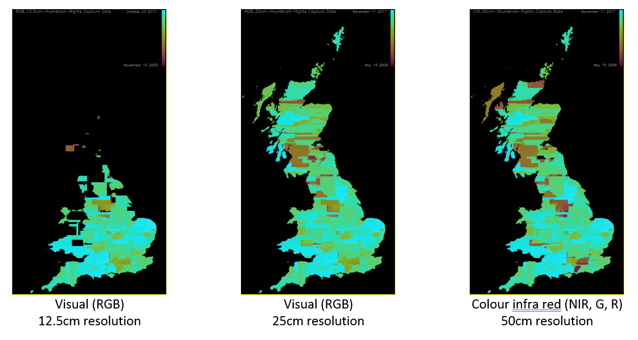
The 12.5 cm RGB images covered October 2005 to September 2017. 133,768 images (23.4 terabytes) were provided each covering a 1 kilometre x 1 kilometre (km) window. Each image consisted of 8,000 by 8,000 pixels. An example 12.5 cm RGB image is given in Figure 3.
The 25 cm RGB images covered April 2006 to October 2017. 244,712 images (10.6 terabytes) were provided each covering a 1 km x 1 km window. Each image consisted of 4,000 by 4,000 pixels.
The 50 cm Colour-infrared (CIR) images covered April 2006 to October 2017. 244,738 images (2.7 terabytes) were provided each covering a 1 km x 1 km window. Each image consisted of 2,000 by 2,000 pixels. An example CIR image is given in Figure 4.
Figure 3: Example 12.5 cm RGB image

Figure 4: Example 50 cm CIR image

A standard RGB spectral representation is used, with the infrared channel mapped to red, the red channel mapped to green and the green channel mapped to blue
File size prohibited storing the imagery as a single file, instead imagery was stored as 1 km x 1 km fixed resolution images based on the OSGB36 datum (an ellipsoid used to approximate the curvature of the earth around GB, with a grid overlaid upon it). For ease of access the images are stored in a hierarchy, for example the 1 km x 1 km cell covering Trafalgar Square (TQ 299 804) is stored as TQ/TQ28/TQ2980.jpg. The least significant digits of the grid point are then used to determine the exact fraction across the image (east, then north). This allows the tiles relating to individual gardens to be quickly and simply retrieved without adding additional platform load.
Data Issues
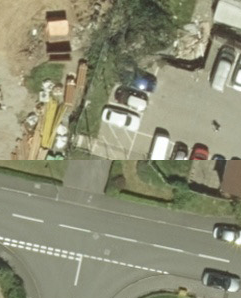
Apart from the obvious challenges associated with storing and processing over 600,000 images relating to nearly 37 terabytes, several other issues were encountered with the data during the course of the project. Visual inspection of the labelled test dataset showed that three of the one hundred images were corrupted or inaccurate to some degree. Figure 5 shows an instance where the garden polygon spans two adjacent gardens belonging to separate properties.
Figure 5: Garden polygon spanning several gardens
First image shows two adjacent properties, the second image highlights the area within the garden polygon, this area clearly spans two gardens.
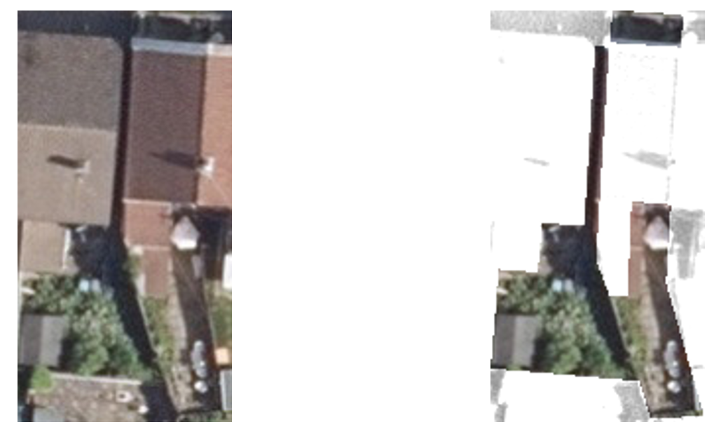
In another image (Figure 6), the garden polygon does not align correctly with the image with sections of the property being included within the polygon and areas of the garden excluded. One image (Figure 7) was found to be corrupted, where image tiles appear to have been incorrectly merged together. In all these cases, the images were removed from the training data and replacement images randomly selected.
Figure 6: Garden polygon misaligned with garden
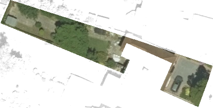
Figure 7: Corrupted image tile
Although not data issues in the strictest sense, there were features within the images that increased the complexity of the classification task. The RGB and CIR images did not cover consistent resolutions, in this case the IR images were upsampled from 50 cm to 12.5 cm. As aerial imagery was captured between April and October, different ground conditions caused discrepancies between areas when the colour profile was cast to CIR. This rendered approaches that require the colour profile to be compared against the infrared channel more sensitive to temporal changes and therefore unfeasible. Finally, as the imagery was taken by aircraft rather than satellites, complete coverage of an area may take several years hence images are likely to be taken at different times of the day and year, they are also subject to the effect of seasonality and changing weather conditions. For instance, images taken late afternoon on a sunny day were more likely to contain shadow, whilst vegetation in gardens suffering from drought conditions are far less likely to be lush green in colour.
3. Vegetation detection
There are many approaches that may be used to detect vegetation in aerial and satellite imagery. These include:
- Red, Green and Blue (RGB) indices including Visual Normalised Difference Vegetation Index (vNDVI)
Green Leaf Index (GLI) and Visual Atmospheric Resistance Index (VARI) - Transformed colour spaces such as Hue, Saturation, Value (HSV) and CEILAB
- Spectral methods such as Normalized Difference Vegetation Index (NDVI)
A comprehensive discussion may be found in Vina and others, 2011 and Xue and others, 2017. The following sections introduce the RGB indices and transformed colour space methods that were investigated in this project.
Visual Normalised Difference Vegetation Index (vNDVI)
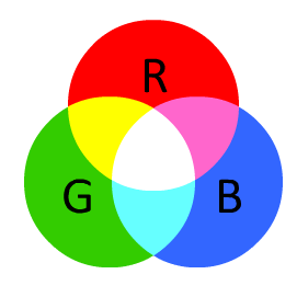
The vDVI algorithm is based upon the Normalised Green Red Difference Index (Rouse and others, 1974). It uses pixels expressed using the RGB spectral channels as shown in Figure 8.
Figure 8: RGB colour palette
The red (R) and green (G) channels of an image are used to calculate an index value, using the following equation,
$$ vNDVI=\frac{(G-R)}{(G+R)}\ $$
The numerator differentiates between plants and soil whilst the denominator normalises for light intensity variations between images. The index ranges from -1 to 1. Individual pixels with values greater than 0 are classified as representing vegetation. vNDVI is a robust and efficient algorithm as it considers only two of the spectral channels however it is sensitive to atmospheric effects, specifically cloud cover.
Green Leaf Index (GLI)
As with vNDVI the GLI algorithm is based upon the RGB colour system, it attempts to distinguish living plants from soil and other matter be identifying the green colour of a healthy plant (Louhaichi, 2001). However, unlike vNDVI, GLI also uses the blue (B) channel,
$$ GLI=\frac{(2 ×G-R-B)}{(2 ×G+R+B)}$$
As with vNDVI, the GLI index ranges from -1 to 1, with negative values representing soil or non-living material and positive values represent living plant material. The green leaf index is less susceptible to atmospheric effects, however as it uses all three spectral channels it is less efficient when compared to vNDVI.
Visual Atmospheric Resistance Index (VARI)
The VARI algorithm again uses the RGB colour system to estimate the fraction of vegetation. Due to its insensitivity to atmospheric effects, it is particularly suited to satellite imagery (Gitelson and others, 2002). It is calculated using the following equation:
$$ VARI=\frac{(G-R)}{(G+R-B)} $$
As with the other two RGB based approaches, VARI ranges from -1 to 1. With positive values indicating vegetation.
Hue, Saturation, Value (HSV)
Unlike the RGB spectral channels where red, green and blue are mixed in an additive way to form a final colour, in HSV colours of each hue (H) are arranged in a radial slice, around a central axis of neutral colours, ranging from black at the bottom to white at the top (see Figure 9). Saturation (S) represents the amount of grey in the colour, with large proportions of grey producing a faded effect. Value (V) works with saturation and controls the brightness of the colour.
Figure 9: HSV colour palette
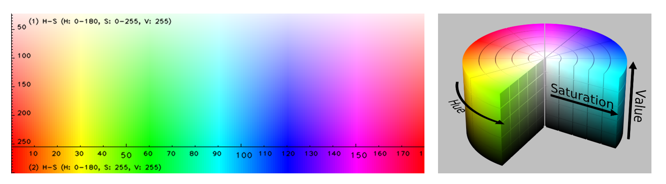 The main benefit of HSV compared to RGB spectral channels is that the colour information for a given pixel is separated from the image intensity, whereas in RGB, colour and intensity are specified by the red, green and blue values. For the purposes of this study a pixel was classified as being vegetation if its hue fell in the range between 30 and 80. Both saturation and value may assume any value in their respective ranges.
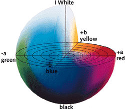
CIELAB (Lab)
The CEILAB colour space expresses colour as three numerical values L represents lightness whilst a* and b* represent the green to red and blue to yellow colour components respectively (see Figure 10). Lab was designed to be perceptually similar to human colour vision where the same amount of numerical change in the L, a* and b* channels correspond to approximately the same amount of visually perceived change.
Figure 10: Lab colour palette
This study applies the threshold values determined in previous work at the Data Science Campus. In this work, the labelled images in the Mapillary Vistas dataset were converted to the Lab colour system. The a* and b* thresholds were then optimised using Bayesian parameter optimisation to maximise the classification of vegetation and urban pixels. The optimal parameters were found to be:
a* channel optimised Lab(a*)
$$ -31 ≤a* ≤-11 $$
a* and b* channels optimised Lab(a*b*)
$$ -31 ≤a* ≤-6 $$
$$ 5 ≤b* ≤57 $$
4. Unlabelled test image library
There is a sizeable amount of literature relating to labelled datasets within street-level imagery, including Cityscapes (Cordts and others, 2016), ADEK20K (Zhou and others, 2017) and Mapilary Vistas (Scharr, 2016). There are also many databases containing general labelled imagery, such as the 15 million high resolution images of ImageNet. Unfortunately, far less work has focussed upon generating databases of labelled aerial imagery identifying areas of vegetation, soil, water and so on. This makes it particularly challenging to identify a comprehensive library of aerial images that can be used to quantitatively assess the performance of the approaches identified in the preceding section.
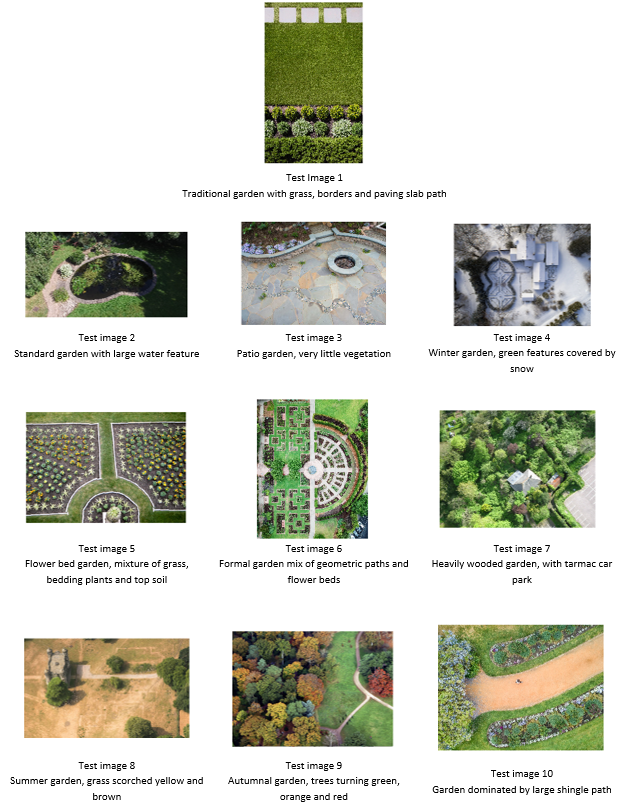
As an initial step, a more qualitative approach was taken. A library of 10 test images were used to empirically investigate the relative performance of each test algorithm. The test library is shown in Figure 11, each image was selected to capture the broad spectrum of garden designs and the seasons upon which the aerial imagery may have been taken, this included:
- garden type (traditional / patio)
- features (ponds, paths, flower beds, trees)
- formality (structured / wild)
- seasonality
Figure 11: The unlabelled test image library
Each test algorithm was applied to the 10 unlabelled test images. In each case the proportion of vegetation identified by each approach was compared against the corresponding test image to give a qualitative view of algorithm performance. A review of all the results is given in the appendix of this report. A selection of the more noteworthy cases is discussed in the next paragraph.
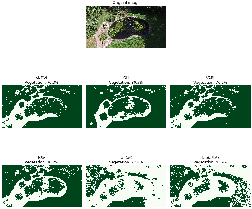
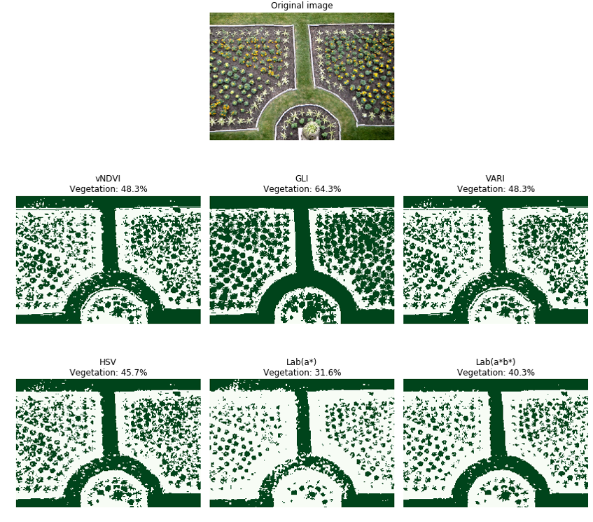
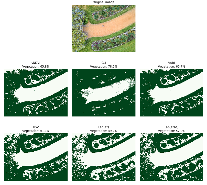
Test image one (Figure 12) explored the ability to identify vegetation in an image of a more traditional garden. All approaches perform well and can accurately identify areas of vegetation. All three of the RGB based algorithms along with the HSV approach are in broad agreement with vegetation coverage ranging from 84-88%. Both Lab approaches have lower values of 73% and 79% for the Lab(a*) and Lab(a*b*) respectively. On closer inspection of the Lab approaches it is evident that Lab(a*) misclassifies some areas of grass at the bottom and top left regions of the image.
Figure 12: Test image 1 results
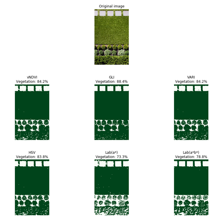
Pixels identified as vegetation are coloured green
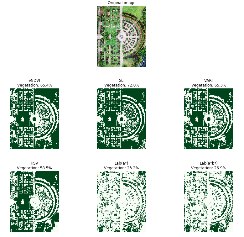
As test image three (Figure 13) contains very limited amounts of vegetation, it can be used to investigate false positive classifications. The RGB algorithms all perform particularly poorly in this instance with the GLI algorithm indicating that the image consists of almost 64% vegetation, this is a clear overestimate. Although not as poor as the RGB algorithms, misclassification is evident in the HSV result, particularly in the lower centre of the image. Conversely both Lab based algorithms perform well suggesting that the image contains only 2.5% and 3.3% vegetation for Lab(a*) and Lab(a*b*) respectively, these figures more accurately reflect the true reality of the image.
Figure 13: Test image 3 results
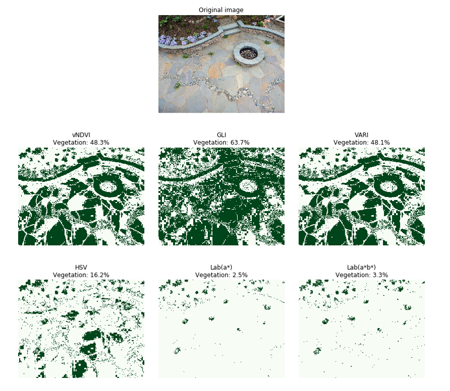
Pixels identified as vegetation are coloured green
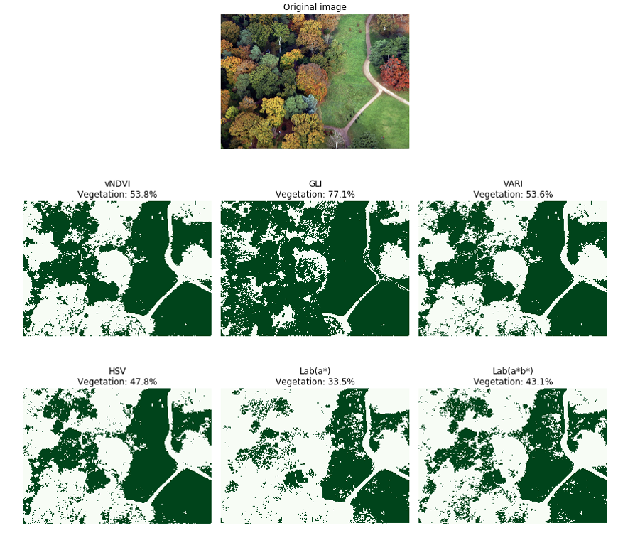
Test image eight (Figure 14) shows a parched garden in which the green grass has turned to predominantly yellow and browner shades. The GLI approach performs particularly poorly here classifying 92% of the image as being vegetation. The performance of all the remaining algorithms are broadly comparable giving vegetation coverage of between 14% to 16%, however Lab(a*) struggles to identify the tree foliage at the lower right and centre of the image.
Figure 14: Test image 8 results
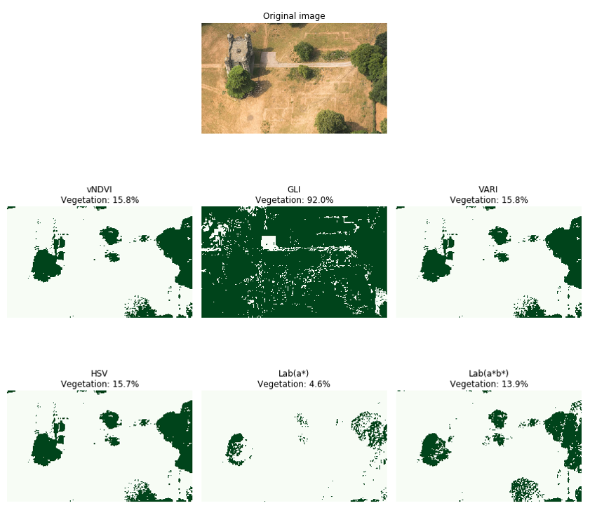
Pixels identified as vegetation are coloured green
Although not definitive, this study illustrates that no single approach performs well across all images in the unlabelled test library. Some approaches perform poorly in images containing patios whilst others struggle to differentiate between areas of water and vegetation.
Although by no means perfect, the performance of Lab(a*b*) and HSV appear to be less sensitive across the range of test images. It is interesting to note that both Lab(a*b*) and HSV apply thresholds to the raw colour channels of the image, rather than thresholding an index calculated from the colour channels as is the case with the remaining approaches.
5. Application to Bristol and Cardiff
The HSV threshold was applied to a selection of real-world images. It appears to perform well, identifying most regions covered in vegetation in Figure 15 – a wider view over Bristol.
Figure 15: Application of HSV approach to Bristol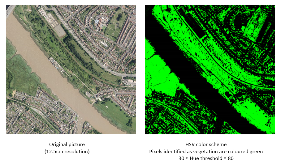
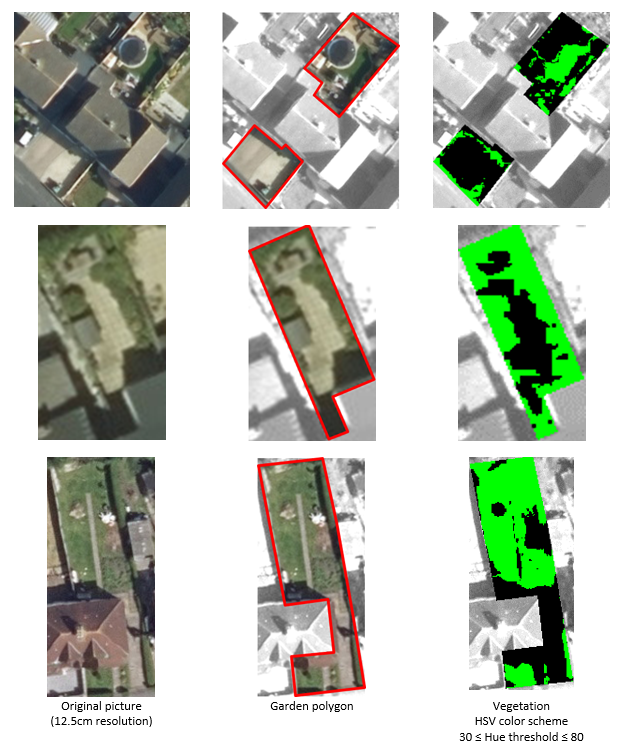
Figure 16 shows a larger scale view of three randomly selected gardens in both Bristol and Cardiff. Although the HSV approach distinguishes between vegetation and urban areas, the performance does not appear to be as impressive as that observed in the higher-level image. There are notable areas of misclassification in all three images; sections of the driveway and the shed are misclassified as being vegetation in the first and second images respectively whilst large areas of vegetation in shadow are missed in the third image. It is suggested that these inaccuracies may be compounded by the lower resolution of the aerial imagery when compared to the images contained within the unlabelled test image library.
An obvious and significant drawback of the images investigated so far is the lack of labelling. Without this ground truth it is impossible to accurately compare performance across approaches or to recommend a preferred approach with any degree of confidence.
This limitation is addressed in the following section.
Figure 16: Application of the HSV threshold to a random selection of Bristol gardens
6. Labelled test image library
Up to this point the test algorithms have been assessed qualitatively on unlabelled test images. Although this approach has increased understanding of algorithm performance its does not allow an objective decision to be made regarding which algorithm gives the optimal performance. To address this a test library of labelled images was created.
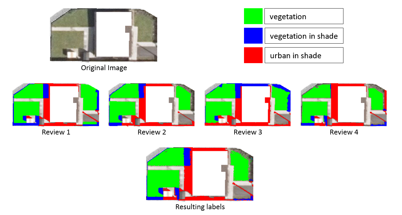
100, 12.5 centimetre resolution aerial images covering gardens in Bristol and Cardiff were randomly sampled and independently reviewed by four individuals. Everyone was randomly assigned 75 images in such a way that each image was reviewed by three people. Each pixel was manually classified into one of the following four categories:
- green – vegetation
- blue – vegetation in shade
- red – urban in shade
- unclassified – urban
Two shaded categories were introduced to explore the relationship between shadow and predictive power and to facilitate the development of supervised learning techniques (see Vegetation detection using supervised machine learning).
To increase accuracy, voting logic was applied, with the overall classification of each pixel taken as the most common classification from the individual reviews (ties were randomly assigned a classification). In this way erroneous classifications were more likely to be “out-voted” by the other two reviews. An agreement matrix was used to illustrate the agreement rate between reviewers and therefore the confidence in the final classifications. If the agreement rate dropped below 80% for any image arbitration was applied and the image was reviewed by a fourth person and the voting logic reapplied. To overcome temporal errors the order of the images was randomised for each reviewer.
The results of the manual review for two images taken from the labelled test image library are given below. For the first image, the agreement matrix indicates very strong alignment across reviewers, with agreement in classification in at least 84% of all pixels within the image. This removed the need for arbitration in this instance (see Table 1). This result is impressive when one considers the complexity of the image being reviewed and demonstrates the power of this approach.
Table 1: Agreement matrix for test image 1
| Review | 1 | 3 | 4 |
| 1 | 85% | 84% | |
| 3 | 85% | 87% | |
| 4 | 84% | 87% |
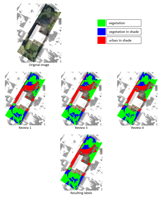
Figure 17 shows the results of the individual reviews and the resulting classified image after voting logic has been applied. The complexity of the classification task is self-evident in the final image. Note that this image has not been reviewed by the second reviewer.
Figure 17: Results of manual review for test image 1
Turning to the second image, the values within the agreement matrix are lower than those in the preceding example (see Table 2). The result is interesting when one considers the more uniform nature of the image.
Table 2: Agreement matrix for test image 2
| Review | 1 | 2 | 3 | 4 |
| 1 | 84% | 56% | 82% | |
| 2 | 84% | 57% | 86% | |
| 3 | 56% | 57% | 54% | |
| 4 | 82% | 86% | 54% |
As the values in the agreement matrix dropped below 75% the image went through arbitration and was reviewed by the fourth person. The results of this and the final post voting logic classification are given in Figure 18. On closer inspection of the final image, a checker board effect is noted in the top right area of the image. This is caused by classification ties and a random choice being made. It is believed that this effect could be reduced by applying a suitable smoothing filter, however as its prominence is slight this was deemed unnecessary.
Figure 18: Results of manual reviewing for test image 2
Application of test approaches to labelled test image library
All six test algorithms were applied to the labelled test image library. In each case the classification error was calculated as:
$$ \small classification \space error = |labelled \space vegetation \space proportion \space – \space observed \space vegetation \space proportion| \ $$
Where “labelled vegetation proportion” is the proportion of vegetation in the labelled dataset and “observed vegetation proportion” is the proportion of vegetation identified by the test algorithm.
A pixel is deemed vegetation if it is either obscured by shadow (coloured blue) or not (coloured green). The results are shown in Table 3, Lab(a*b*) provides the best approach with an average classification error of 16.3% with HSV in second place with an error of 20.7%.
The comparable high performance in both HSV and Lab(a*b*) approaches are in general agreement with those of the qualitative assessment on the 10-image unlabelled test library.
Table 3: Classification error across all 100 labelled images, sorted in ascending classification error
| Average | StdDev | |
| Lab(a*b*) | 16.3% | 14.8% |
| HSV | 20.7% | 18.4% |
| vNDVI | 23.2% | 17.7% |
| VARI | 23.2% | 17.7% |
| Lab(a*) | 31.3% | 19.2% |
| GLI | 39.5% | 27.9% |
| Naive | 60.2% | 24.0% |
The Naïve approach assumes all areas falling within the residential garden polygon are vegetation.
An interesting finding is noted if the results are broken down by region. Lab(a*b*) performs relatively poorly when applied to Bristol urban residential gardens (coming fifth out of the six approaches) whilst performing exceptionally well in Cardiff urban residential gardens. The HSV algorithm performs broadly well across both regions.
Table 4: Classification error across all 100 labelled images, broken down by Bristol and Cardiff, sorted in ascending classification error
Bristol
| Average | StdDev | |
| HSV | 13.5% | 14.6% |
| vNDVI | 15.4% | 12.6% |
| VARI | 15.4% | 12.6% |
| GLI | 19.1% | 13.5% |
| Lab(a*b*) | 22.4% | 16.7% |
| Lab(a*) | 34.2% | 19.9% |
| Naive | 57.9% | 24.6% |
Cardiff
| Average | StdDev | |
| Lab(a*b*) | 10.1% | 9.4% |
| HSV | 28.0% | 19.2% |
| Lab(a*) | 28.5% | 18.1% |
| vNDVI | 30.9% | 18.8% |
| VARI | 30.9% | 18.8% |
| GLI | 59.8% | 23.4% |
| Naive | 62.5% | 23.4% |
The Naïve approach assumes all area falling within the garden polygon is vegetation
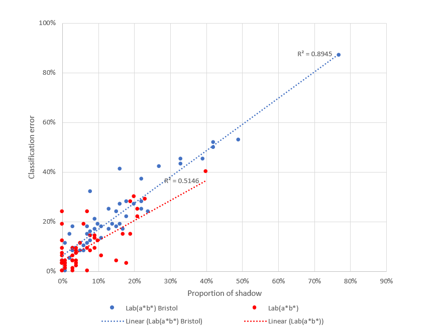
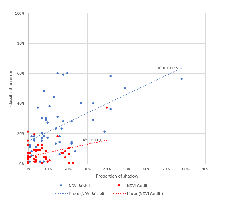
This difference in performance of Lab(a*b*) across both regions may be caused by a sensitivity to shadow. Across the labelled test images the average proportion of vegetation covered by shadow was 15% in Bristol and 7% in Cardiff. The images where Lab(a*b*) performs poorly are those images that are subject to the highest proportion of shadow. Figure 19 and Figure 20 show the relationship between classification error and proportion of shadow (pixels classified as either red or blue) for HSV and Lab(a*b*) for all images in the training and test datasets. For Bristol gardens where shadow is more evident, the R-squared values are 0.84 and 0.89 for HSV and Lab(a*b*) respectively. Turning to Cardiff, classification again increases with increasing shadow for Lab(a*b*) with an R-squared of 0.51, however error decreases for HSV with an R-squared of -0.22.
In both cases Lab(a*b*) seems to be more sensitive to shadow, this may be explained by the fact that the Lab approaches were calibrated using street level imagery where the shadows would be less prominent when compared to the aerial imagery used in this study.
Figure 19: Relationship between classification error and shadow for HSV (Bristol and Cardiff gardens).
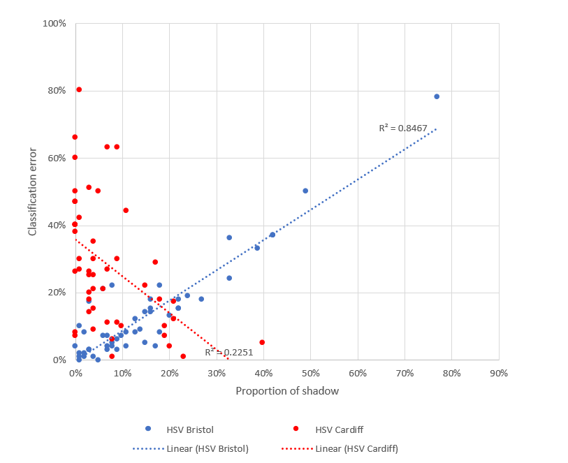
Figure 20: Relationship between classification error and shadow for Lab(a*b*) (Bristol and Cardiff gardens)
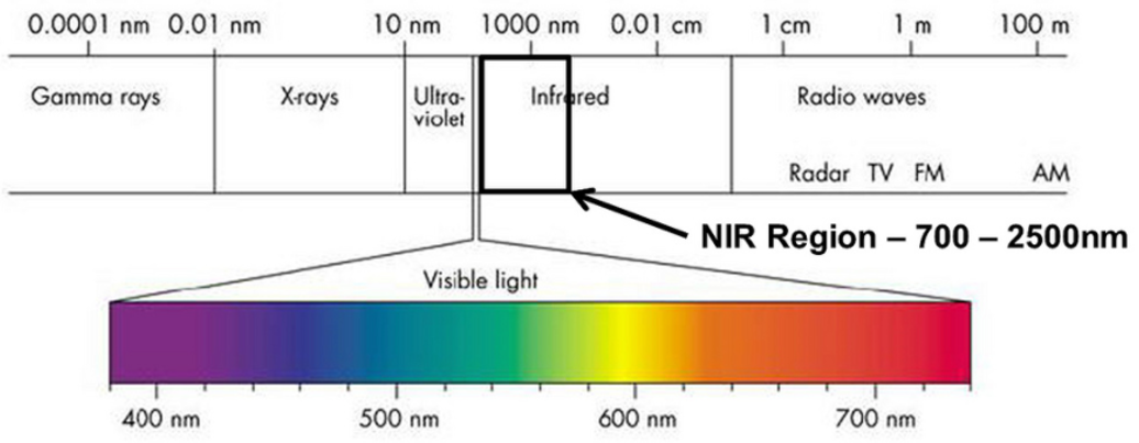
7. Vegetation detection using infra-red spectral bands
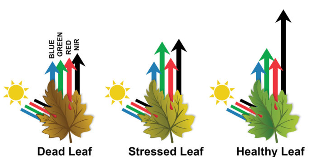
Light from the sun in the form of electromagnetic radiation includes wavelengths that are both visible (red, green and blue spectral channels) and invisible (ultra-violet and infrared channels). As well as visible light, aerial imagery can detect invisible light from the infrared part of the spectrum with the shortest wavelengths, termed the Near Infrared (NIR). When Near Infra-Red (NIR) light (Figure 21) hits organic matter containing chlorophyll the red part of the colour spectrum is absorbed and the NIR part is reflected. Hence the relationship between the red and NIR channels can be used to determine if a pixel corresponds to organic matter (Rouse and others, 1974).
Figure 21: Electromagnetic spectrum highlighting the visible and Near infra-red regions
The NIR imagery used for this project was provided as 50 centimetre resolution colour infra-red images consisting of NIR, red and green channels. Each image tile covered the same geographic area as the 12.5 cm resolution RGB images. The NIR channel was extracted and interpolated to 12.5 cm resolution and combined with the RGB images to produce 12.5 cm resolution four channel NIR, R, G, B images.
NDVI
The Normalised Difference Vegetation Index (NDVI) calculates the normalised difference between the red and infrared bands for quantitative and standardised measurement of vegetation presence and health (Deering and others, 1975). Healthy vegetation has a high reflectance of Near-Infrared wavelengths and greater absorption of red wavelengths due to a greater chlorophyll composition (see Figure 22).
The Near-Infrared (NIR) and red (R) spectral channels of an image are used to calculate an index value, using the following equation,
$$ NDVI=\frac{(NIR-R)}{(NIR+R)} $$
The index ranges from -1 to 1. In this study, individual pixels with a value greater than 0 are classified as vegetation due to their higher reflectance of Near-Infrared. The closer to 1 the healthier the vegetation and greatest density of green leaves. vNDVI, in a similar manner to NDVI, is also sensitive to atmospheric effects, specifically cloud cover and should be atmospherically corrected when used in studies analysing change over time.
Figure 22: Reflection and absorption of wavelengths in healthy/unhealthy vegetation
The results of applying NDVI to the 100 labelled images are compared against Lab(a*b*) and HSV in Table 5. The use of the infra-red band in the NDVI approach appears to offer slight improvement over the dual threshold Lab approach (classification error of 15.6% compared to 16.3%), however this comes with a reduction in robustness indicated by the standard deviation of classification error.
Table 5: Classification error across all 100 labelled images for NDVI, Lab(a*b*) and HSV, sorted in ascending classification error
| Average | StdDev | |
| NDVI | 15.6% | 15.5% |
| Lab(a*b*) | 16.3% | 14.8% |
| HSV | 20.7% | 18.4% |
If the results are broken down by region (Table 6), NDVI performs exceptionally well in Cardiff (where only 7% of the images are covered in shadow, but relatively poorly in Bristol with its greater proportion of shadow (15%).
Table 6: Classification error across all 100 labelled images for NDVI, Lab(a*b*) and HSV, broken down by Bristol and Cardiff and sorted in ascending classification error
Bristol
| Average | StdDev | |
| HSV | 13.5% | 14.6% |
| Lab(a*b*) | 22.4% | 16.7% |
| NDVI | 24.5% | 16.8% |
Cardiff
| Average | StdDev | |
| NDVI | 6.8% | 6.6% |
| Lab(a*b*) | 10.1% | 9.4% |
| HSV | 28.0% | 19.2% |
Further evidence of the sensitivity of NDVI to shadow can be seen in Figure 23. Here it can be seen that classification error increases with increasing proportion of shadow in the labelled images for both Bristol and Cardiff.
Figure 23: Relationship between classification error and shadow for NDVI (Bristol and Cardiff gardens).
This result and similar results with HSV (Figure 19) and Lab(a*b*) (Figure 20) illustrate the sensitivity of the solutions investigated so far to the effects of shadows. It is clearly unavoidable that aerial imagery will be subject to differing amounts of shadow as images may be taken at different times of the year, times of the day or on days where the weather conditions vary considerably. It follows that any approach used to extract information directly from such images should be as insensitive as possible to the effect of shadow. An approach to achieve this using supervised machine learning is discussed in the following section.
8. Vegetation detection using supervised machine learning
The use of machine learning to classify remote imagery is an ongoing area of interest. Generally, approaches focus upon either unsupervised learning where algorithms such as autoencoders are used to learn a set of representation directly from the data (Vincent and others, 2008, Firat and others, 2014) or by applying pre-trained supervised learning techniques such as Convolutional Neural Networks (CNN) to classify each image into a unique category such as buildings, tennis courts, harbours and so on (Marmanis and others, 2016).
Armed with a labelled image library, a supervised machine learning classifier was trained to specifically classify each pixel into one of the three labelled classes. The core inputs to the classifier included the standard RGB spectral channel values that describe the pixels. These inputs were further supplemented by firstly, a number of principal component-based features that specifically reduce the presence of shadows and secondly, an infra-red feature that can be used to identify the presence of chlorophyll. An additional classifier that uses the near infra-red spectral channel is also discussed.
Principal component-based features
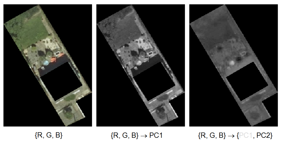
Principal component analysis (PCA), is an established technique for reducing the dimensionality of multiple spectral channels (JARS, 1993). More recently PCA has been used to remove shadows from surveillance images (Shin and others, 2000). Its application here is best explained by example. The image in Figure 24 shows a garden represented by the standard RGB colour channels. The building in the centre of the image projects a large shadow from its northern edge. If PCA is used to reduce the three channels to a single channel the resulting image may be shown monochromatically (second image of Figure 24), however the shadow is still present as it has been captured by the single principal component. However, if the three channels are reduced to two principal components, the first component will correspond to the strongest source of contrast within the image, which although not guaranteed, is most likely to relate to shadow. The stronger component can then be discarded, and the second weaker component represented as a monochromatic image (third image of Figure 24). In this instance is can be seen that the intensity of the shadow has diminished significantly.
Figure 24: Principal component analysis used to reduce an RGB image to a single monochromatic channel
This technique is developed further by taking comparable channels from the RGB, HSV and Lab spectral channels, extracting the first four principal components to remove the linear relationships between similar spectral channels and discarding the first component that contains shadow elements.
Figure 25 shows this approach applied to a sample garden. In the second image the channels that relate to image brightness are used, specifically the three channels from RGB, the value (V) channel from HSV and the lightness (L) channel from Lab. In the third image the colour related channels are used, the three channels from RGB, the hue (H) channel from HSV and the a and b channels from Lab. In both cases the first four principal components are extracted, and the first component discarded. The three remaining principal components can be visualised by mapping to a standard RGB representation. This mapping is arbitrary, however, it does give a general feel for the difference between the brightness and colour based principal components.
The shadow reducing principal components approach discussed here shares a similarity to the feature maps generated by CNNs (LeCun and others, 1998), where each map captures different characterises inherent within the image.
Figure 25: Principal component analysis used to reduce an RGB image to a brightness and colour channels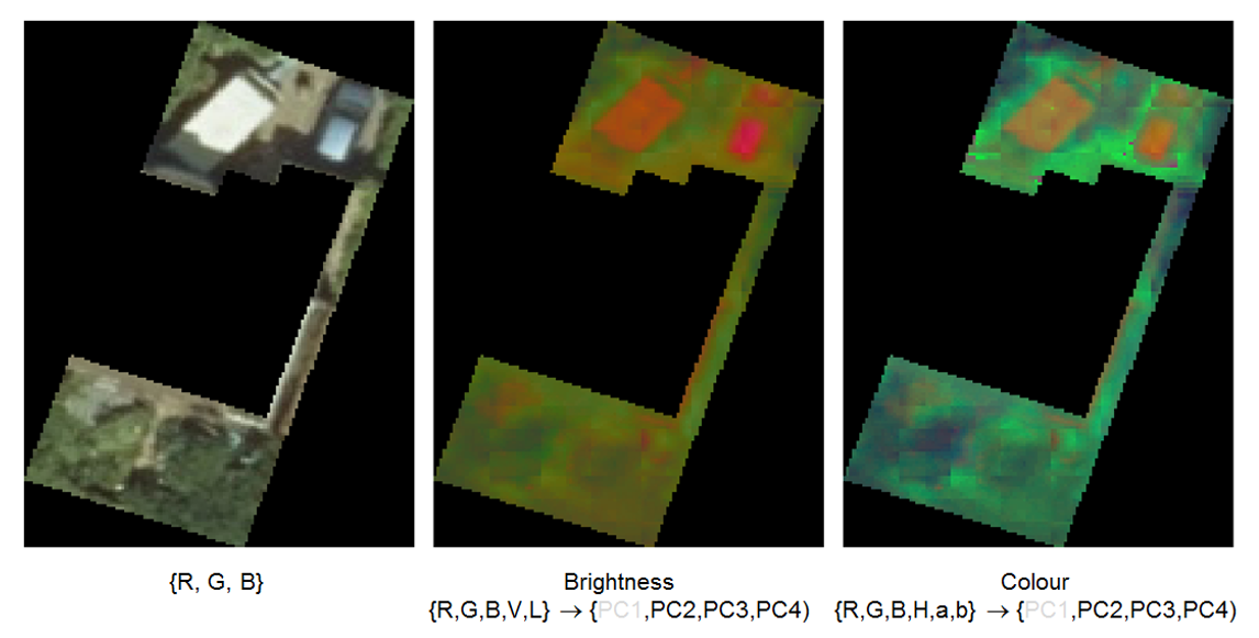
PC2 mapped to the red channel, PC3 mapped to the green channel and PC4 mapped to the blue channel
Neural network classifier
In general, image-based classifiers work by using the spectral characteristics of a pixel, such as the Red, Green and Blue channel values to assign a classification to one or more known land cover classes. The challenge arises in determining a similarity measure that can be used to determine the most appropriate class.
Approaches range from simple Euclidean distance (Richards and Jia, 2006) to the more involved spectral angle mapping (Kruse and others, 1993) and parallelpiped (Richards and Jia, 2006) approaches. The approach presented here uses an Artificial Neural Network (ANN) to classify pixels into one of the following four categories:
- vegetation
- urban
- vegetation in shade
- urban in shade
The labelled image library was randomly sampled into training and test datasets in an 80:20 ratio, the samples were stratified to ensure equal representation from Bristol and Cardiff urban residential gardens (Table 7). Although the training data consisted of only 80 images; the pixels were treated independently so the training dataset contained over 880,000 records.
Table 7: Train and test dataset sizes
| Train | Test | |||
| Images | Pixels | Images | Pixels | |
| Bristol | 40 | 514,531 | 10 | 136,948 |
| Cardiff | 40 | 368,670 | 10 | 104,995 |
| 80 | 883,201 | 20 | 241,943 | |
The neural network contained four outputs (each relating to one of the classes) and the following eleven inputs:
- the three RGB spectral channels
- the single monochromatic principal component with first component (assumed to be shadow) removed
- the three brightness principal components with first component (assumed to be shadow) removed
- the three colour principal components with first component (assumed to be shadow) removed
- the single NIR spectral channel
All inputs were scaled to consistent distributions. A 20% validation dataset was used to terminate search before overtraining occurred. Various network architectures were explored using a randomised grid search, with a three layer 12:8:4 network giving the optimal performance. Standard rectified linear (ReLU) activation units were used in all but the output layer, where a softmax function was used to ensure all outputs summated to 1. Learning terminated with training and validation errors of 0.819 and 0.792 respectively.
The resulting network was used to classify the 20 images of the test dataset. The manual and predicted labels for three images taken from the test dataset are shown in Figure 26. Here it can be seen that the neural network performs well and matches the manual classification in many areas. However, there are areas where the network fails to correctly classify pixels, specifically in the first image significant areas in the lower region are classified as red (urban in shade), where the assumed correct label is blue (vegetation in shade), further instances of these are evident in the two remaining images of Figure 26.
There also appears to be areas where the network struggles to differentiate between vegetation and vegetation in shade, the lower region of the third test image is a notable example of this. In this instance the mismatch between the predicted and actual labels appear to be exasperated by the presence of the tree canopy resulting in a patch work of small regions of vegetation in and out of shade.
Figure 26: Manual and predicted labels for three images from the test dataset
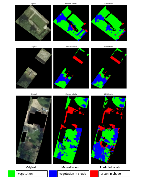
A further drawback of the neural classifier is that it treats pixels in isolation and does not consider neighbouring pixels. Where a human observer would make the logical assumption that if all the pixels surrounding a given pixel relate to vegetation, then it is likely that the pixel itself will also be vegetation. The classifier will not detect this, instead it will make the classification based entirely upon the characteristics of that pixel. This drawback is particularly evident in areas with a dominant classification. The diagonal red area in the second row and the top left green area of the third row in Figure 26 are examples of this.
The performance of the neural network is compared with the other test algorithms in Table 8 and broken down for Bristol and Cardiff in Table 9. The first point of note is that the values differ from the results in Table 3 and Table 4, this is caused by the different test dataset sizes with the previous assessment being made across all 100 images in the test library and assessment here being made upon the 20 image test dataset.
Table 8: Classification error across all 20 labelled test images (sorted in ascending classification error)
| Average | StdDev | |
| ANN | 7.7% | 7.2% |
| NDVI | 17.2% | 16.8% |
| Lab(a*b*) | 18.6% | 21.4% |
| HSV | 19.7% | 21.7% |
| vNDVI | 21.0% | 14.7% |
| VARI | 21.0% | 14.7% |
| Lab(a*) | 36.7% | 19.8% |
| GLI | 37.1% | 22.3% |
| Naive | 51.3% | 22.2% |
The neural network classifier outperforms the NDVI, Lab(a*b*) and HSV approaches, with classification errors being reduced by factors of 2.2, 2.4 and 2.6 respectively. The standard deviation is also significantly reduced, reflecting the increased robustness of the machine learning approach.
Table 9: Classification error across all 20 labelled test images, broken down by Bristol and Cardiff (sorted in ascending classification error)
Bristol
| Average | StdDev | |
| ANN | 6.3% | 7.0% |
| vNDVI | 16.0% | 8.1% |
| VARI | 16.0% | 8.1% |
| HSV | 17.6% | 26.0% |
| GLI | 24.5% | 15.6% |
| Lab(a*b*) | 28.6% | 26.3% |
| NDVI | 28.9% | 16.8% |
| Lab(a*) | 41.3% | 23.3% |
| Naive | 49.4% | 22.8% |
Cardiff
| Average | StdDev | |
| NDVI | 5.5% | 2.9% |
| Lab(a*b*) | 8.6% | 7.4% |
| ANN | 9.0% | 7.6% |
| HSV | 21.7% | 17.6% |
| vNDVI | 26.0% | 18.3% |
| VARI | 26.0% | 18.3% |
| Lab(a*) | 32.0% | 15.4% |
| GLI | 49.7% | 21.3% |
| Naive | 53.1% | 22.6% |
If the results are further broken down by region its can be seen that in the Cardiff images where shadows were less evident, the performance of the neural network classifier is:
- weaker than NDVI,
- on a par with Lab(a*b*)
- significantly better than all other approaches
Considering the results for Bristol (with greater proportions of shadow), the performance of both NDVI and Lab(a*b*) are significantly poorer and outperformed by the majority of the remaining test approaches.
The neural network significantly out performs all other test approaches as it is better able to cope with the difference in the imagery of both Bristol and Cardiff. As the deployed algorithm is to be applied to imagery taken from different regions and at different times of the day and year, it is concluded that the neural network offers the best compromise between performance and the robustness to classify vegetation under changing local conditions.
9. Deployment
Considerable effort was placed on developing a robust, efficient and scalable pipeline to deploy the investigated algorithms to large volumes images, the approach developed is discussed below.
The source code is available in a public GitHub repository.
Configuration
A JSON file is used to store available image loaders and vegetation classification approaches. Each image loader defines the spectral channels for a given image (for instance R, G, B or Ir, R, G), the location of the data, the dataset name and the python class responsible for loading the data. This enables new image loaders to be added without changing existing code, with specific image loaders having additional parameters as required. For instance, Ordnance Survey (OS) national grid datasets have a specific number of pixels per 1 kilometre (km) square (determined by image resolution, for example 12.5 centimetre (cm) imagery is 8,000 pixels wide). This enables a resolution independent Ir, R, G, B data reader to be created that internally combines the CIR and RGB datasets to generate the required imagery on demand.
The data sources are intentionally independent of the vegetation indices. Additionally, the same data reader can be used with different physical datasets. For example, 25 cm OSGB data can be read using the same reader as 12.5 cm OSGB data, with a minor configuration change needed specifying the location of data and number of pixels per image. As the data readers are python classes with the same methods, the code that uses a reader does not need to know if it is consuming OSGB data or Web Mercator, it simply uses the returned results which are in a common form and hence source agnostic.
The vegetation indices are defined in the JSON file to enable the end user to add new metrics and change their thresholds without altering Python source code. Metrics may be from a different codebase entirely rather than restricted to be part of the project source code. Vegetation indices and image loaders are defined in terms of class name and created using Python’s importlib functionality to create class instances directly from names stored as text strings at run time. Geometries are passed as a command line argument (using argparse) for processing, along with the dataset to use and the index to be calculated (both named in the JSON configuration).
GeoJSON reader
The standard JSON reader is used to read the GeoJSON data, and the garden polygons are extracted (see Figure 27).
Polygon extraction and projection
Polygons are held within a dictionary. A standard loop iterates over the data file and extracts data stored against the specific geometry key. The image loader is a python class that can convert a polygon defined in terms of latitude and longitude into its local coordinate system. The transforms are stored as separate functions in a coordinate transforms library where they can be reused by different image loaders. The transformations use the pyproj library (a Python wrapper for the proj.4 library) to convert between standard geospatial coordinate systems.
Figure 27: Deployment process flow diagram
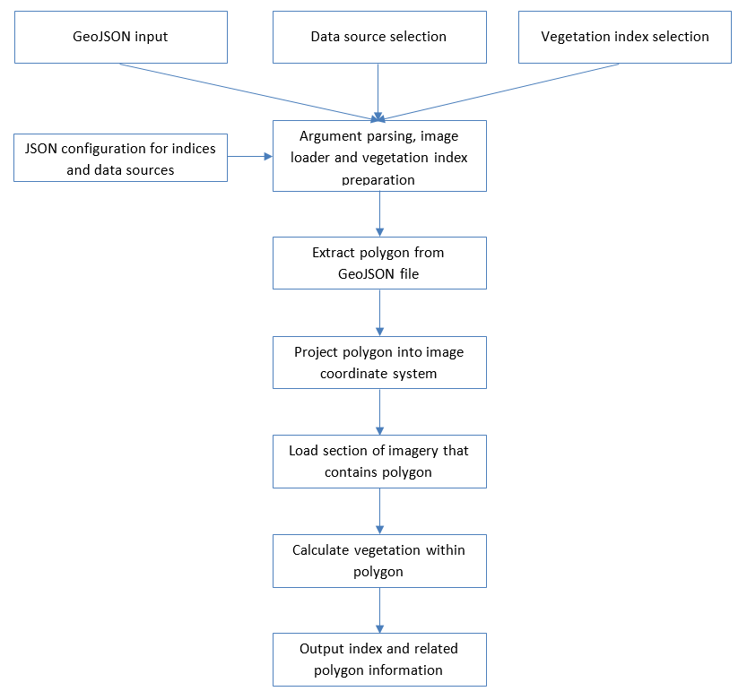
Image extraction
The bounding box containing the projected polygon is calculated and the footprint of the polygon is used to calculate what image tiles need to be loaded. The image loaders import the required tiles (using the raster library) and merge the tiles together to form a large, continuous image that is then cropped to only contain the bounding box.
A mask image is then generated that is the same size as the cropped image, but the projected polygon is drawn on the mask image such that pixels within the polygon are set to ‘true’ otherwise ‘false’ (using the shapely library). This indicates which pixels in the cropped image are to be analysed later by the index calculation code.
A major overhead in processing is downloading and decompressing the image files. To improve efficiency and reduced processing time, image tiles that are loaded are cached for reuse (via the method decorators in the cachetools package).
Vegetation Indices
All vegetation indices are defined as python classes that extract their configuration directly from the JSON configuration file, enabling unique configuration options for each class. All classes implement an index method that accept the related cropped image bitmap, enabling the main codebase to use index classes interchangeably. The codebase has no dependency upon implementation. The index method iterates over pixels in the cropped image bitmap, using OpenCV and NumPy to import images and speed up processing respectively. A bitmap is returned where 1 indicates that a pixel represents vegetation and 0 otherwise.
The cropped image is processed in its entirety to simplify implementation of the index method and to utilise the vector processing support enabled by NumPy. The main code base combines the mask bitmap with the resulting vegetation bitmap to calculate the vegetation coverage for the given garden polygon.
Process timings
To produce the final statistics for Cardiff and Bristol, the Neural Network classifier was used with the 12.5 centimetre RGB data combined with 50 cm IR to generate 12.5 cm RGBIr data. The Cardiff data (79,643 polygons) was processed with a two-core virtual machine hosted on a Xeon E5-2650 @ 2.20 GHz; 4 Gigabytes of memory was allocated for caching which resulted in 99.6% cache hit rate to analyse the gardens in 12 hours and 45 minutes. The Bristol data (209,035 polygons) was run on a two-core virtual machine hosted on a Xeon Gold 6126 @ 2.60GHz; 28 Gb of memory was allocated for caching which resulted in 70% cache hit rate but had taken 31 hours to process less than 50% of the data. This was too slow to be of use, so the Bristol run was aborted.
To reduce the problem of cache misses, pre-sorting code introduced where each polygon was projected onto the aerial imagery and its related image tile calculated. Polygons are then processed in order of image tile, to maximum image reuse. This has resulted in a cache hit rate of 99.9% with the Bristol gardens and final execution reduced to 29 hours and 38 minutes. Approximately 11 Gb of memory was used for caching out of 28 Gb made available.
Testing
The code is tested using PyTest, verifying that the image transformation, image loaders and vegetation indices operate as expected. Further, Travis-CI integrated with GitHub is used to ensure that the tests are run as continuous integration to ensure the stability of the code.
Codebase reuse
The existing codebase has no dependency on the concept of gardens or vegetation; it simply processes polygons and runs metrics over projected polygons. The code is therefore not restricted to vegetation coverage in gardens and could be applied to property polygons and metrics to calculate roof types, or farmland polygons with metrics to calculate crop types, hence the code is not restricted to vegetation coverage in gardens.
10. Final Results
Applying the trained neural network to urban residential gardens in Cardiff, Bristol and then for the whole of Great Britain, the total garden area and vegetation coverage is shown in table 10.
Table 10: Total urban garden area and percentage of vegetation
| Area | Total garden area (km2) | Vegetation coverage |
| Cardiff | 13.4 | 53.9% |
| Bristol | 41.9 | 45.0% |
| Great Britain | 61.6% |
11. Practical applications
The neural network classifier detailed in this report will be used by both the natural capital team at the Office for National Statistics (ONS) and Ordnance Survey (OS).
ONS Natural capital team
Natural capital is the term encompassing all the UK’s natural assets that form the environment in which we live. The Natural Capital team at the ONS aims to measure the environment and its relationship with the economy. The team covers measurement in three main areas:
- Environmental flows – the flows of natural inputs, products and residuals between the environment and the economy, and within the economy, both in physical and monetary terms.
- Stocks of environmental assets – the stocks of individual assets, such as water or energy assets, and how they change over an accounting period due to economic activity and natural processes, both in physical and monetary terms.
- Economic activity related to the environment – monetary flows associated with economic activities related to the environment, including spending on environmental protection and resource management, and the production of “environmental goods and services”.
Uses for vegetation classifier include:
- Estimate the benefits of sustainable urban drainage (SUDS) such as vegetation. This would involve discussion with The Environment Agency and devolved equivalents about their own flood risk mapping and how these data might alter risk.
- Improving the calculation of Urban heat by including vegetation coverage and identifying areas where encouraging greener gardens may improve lives.
- Models are currently being developed to predict house prices, the current source of giving green spaces coverage is less accurate and may be replaced.
- Granular carbon sequestration – differentiate between trees and grass and understand how this may impact the carbon footprint at an individual household level.
Ordnance Survey
The degree of surface naturalness is increasingly in demand among Green Infrastructure studies as intelligence beyond the vector garden boundary is lacking. Although an asset often belonging to a singular residence, these high-quality natural spaces are a key deliverable of the 25-year environment plan to increase engagement with the natural environment.
In a previous piece of work in accessing the Greater Manchester Combined Authority’s accessible natural greenspace, residential garden greenspace was used in its naïve entirety which contributed towards an overestimation of natural land cover when analysing land use across larger geographies. This refined insight is intended to provide robust statistics that can therefore improve estimations of greenspace coverage.
The Welsh Government also rely upon quality green infrastructure data to implement multiple policies and schemes – such as the Physical Environment domain within the Welsh Index of Multiple deprivations (WIMD) and the Understanding Welsh Places study.
In its infancy in 2019, the natural green space sub-domain will seek to acknowledge these data refinements into future iterations of WIMD to produce the most accurate account of accessible and ambient greenspace as possible. Beyond the core remit of this project it is hoped that the transferable methodologies from this work can continue to help support and underpin policies surrounding accessibility and quality of natural capital such as the Play Policy to increase Welsh Governments alignment to the United Nations Convention on Rights of the Child.
12. Summary
This report details the work undertaken at the ONS Data Science Campus, in collaboration with Ordnance Survey (OS) to use remote sensing and machine learning techniques to improve upon the current approach used within the ONS to identify the proportion of vegetation for urban residential gardens in Great Britain.
Data was provided in the form of garden parcel polygons covering Cardiff and Bristol, and aerial imagery at 12.5, 25 and 50 centimetre resolution using the RGB and near infra-red spectral channels.
Several “off the shelf” and bespoke techniques developed by both the Campus are used to detect the presence of vegetation. They were assessed qualitatively on a library of 10 garden images, selected to reflect the spectrum of garden designs and changing conditions. It was found that no single approach performed well over all the unlabelled test images. Some approaches performed poorly in images containing patios whilst others struggled to differentiate between areas of water and vegetation. Although by no means perfect, the performance of two approaches Lab (a*b*) and more notably HSV appear to be less sensitive across the range of test images.
Although the 10 images of the unlabelled library allowed a subjective assessment across the algorithms to be made, it did not provide enough quantitative evidence to make a definitive decision.
To overcome this, a second test library of labelled images was created by taking 100 images randomly sampled from Bristol and Cardiff. These were independently labelled by a team of four individuals from the Campus and Welsh Government to provide ground truth.
Application of the test algorithms to the labelled data shows the sensitivity of the test algorithms to shadows, with HSV performing well in images with more shadow whilst Lab(a*b*) performed poorly. Conversely in images subject to less shadows Lab(a*b*) was the clear winner.
A neural network was developed to assign pixels into one of the four classes, the inputs to the network were the standard RGB spectral channels, a NIR channel and a number of monochrome, brightness and colour based principal components with the first component (most likely to be shadow) removed. The performance of the neural network was compared to the test algorithms on a 20-image labelled test library. Results support the conclusion that a neural network classifier can accurately classify vegetation and less susceptible to the effect of shadows when compared with the other test algorithms.
Finally, a robust, efficient and scalable pipeline to deploy the investigated algorithms to any number of images.
13. Future work
There are many areas where the work discussed in this report may be developed or improved.
Firstly, the size of the labelled training dataset should be increased. In the machine learning approach deployed in this report, where pixels were treated in isolation there were enough training examples (over 800k) to train a classifier. However, if more complex networks are explored (such as convolutional networks) where pixels are not treated in isolation a training set of 100 images will be totally inadequate.
In the neural network approach described above, each pixel is treated in isolation, this was found to have a significant drawback. It is clear that if all the pixels surrounding a pixel are vegetation, then it is likely that the pixel itself will also be vegetation. The classifier will not detect this, instead it will make the classification based entirely upon the characteristics of the pixel. Features relating to the neighbouring pixels as potential network inputs should be investigated.
Within all the test algorithms the threshold that determines if a pixel is classified as being vegetation was set at an initial value and not changed. With the availability of labelled data, the thresholds should be recalibrated, to optimally classify the ground truth labels and provide a fairer test against the developed neural network classifier.
Finally, the detrimental effect of shadow upon performance has been shown in this report. The degree of shadow is dependent upon the prevailing weather conditions, the time of the day and the month of year in which the aerial imagery was captured. Given sufficient training data, these additional features may allow the neural network to determine the degree of shadow in the image and therefore automatically correct for this whilst making its prediction.
14. Acknowledgments
Authors: Christopher Bonham, Sonia Williams, Ian Grimstead (ONS Data Science Campus) and Matt Ricketts (Ordnance Survey).
The participants of this project would like to thank the Geography & Technology Team within the Welsh Government for providing resource that contributed towards the aerial imagery labelling aspect of this project, and the Geography team at the ONS for facilitating the provision of the data. The invaluable input and direction from the Natural Capital team at the Office of National Statistics was also greatly appreciated.
15. Appendix: Application of the test algorithms to the unlabelled test image library
The second test image explores the ability of the detection algorithms to distinguish between water, grass and shade (Figure 28). Regarding identified vegetation, the Red, Green and Blue (RGB) and Hue, Saturation, Value (HSV) algorithms are in close agreement, however all of these approaches misclassify both the garden pond at the centre of the image and regions of shade at the right of the image as vegetation, with the Green Leaf Index (GLI) algorithm being particularly poor. The Lab algorithms identify far less vegetation with both Lab(a*) and more notably Lab(a*b*) being able to distinguish between water and the green plants floating upon it. The Lab approaches are also more successful in discriminating between areas of vegetation and shade.
Figure 28: Test image 2 results
Pixels identified as vegetation are coloured green
As with the previous image, test image 4 (Figure 29) contains very limited vegetation. This being caused by snow which covers large areas of grass but leaves shrubs and tree foliage unaffected. This test image produces extreme results. For two of the three RGB based algorithms, significant portions of snow are incorrectly classified as vegetation with values of 60%. Conversely the two Lab approaches identify almost no vegetation (less than 1% in both cases). HSV offers an improvement upon this but this is only marginal. The remaining RGB algorithm, GLI, offers the best performance by far discriminating successfully between areas of snow and vegetation.
Figure 29: Test image 4 results
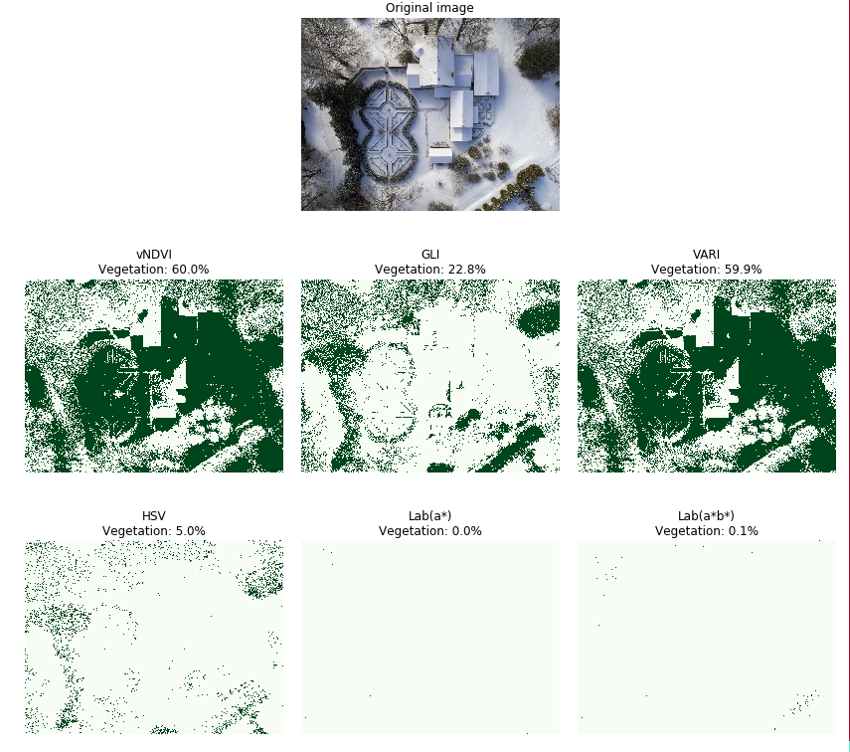
Pixels identified as vegetation are coloured green
Test image 5 (Figure 30) represents a flower bed garden with a mixture of grass, bedding plants and top soil. All the techniques perform well. However, the GLI approach appears better able to identify the both the semi-circular grass border at the bottom of the image and the bedding plants. Conversely, Lab(a*) struggles to identify large portions of the same border.
Figure 30: Test image 5 results
 Pixels identified as vegetation are coloured green
Test image 6 (Figure 31) is an ornamental garden with formal flower beds and geometric walkways. The results here are similar to those observed for test image 5, however in this case both Lab instances perform less well with both failing to identify areas of grass most notably in the top right-hand corner of the image.
Figure 31: Test image 6 results
 Pixels identified as vegetation are coloured green
Test image 7 (Figure 32) tests for the ability to classify vegetation in the form of tree foliage. All three RGB based algorithms and the HSV algorithm achieve this however they misclassify the roof at the centre of the image as also being vegetation. HSV identifies the tree canopy but also can correctly distinguish between the trees and the building roof. Both Lab approaches and more notably Lab(a*) struggle to accurately classify all the tree canopy as green, struggling with the lighter green shades.
Figure 32: Test image 7 results
 Pixels identified as vegetation are coloured green
In test image 9 (Figure 33), Visual Normalised Difference Vegetation Index (vNDVI), Visual Atmospheric Resistance Index (VARI) and HSV all perform well and are able to classify the grass in the centre of the image and the tree canopy on the left of the image (struggling only with the more autumnal shades or orange and yellow). GLI also performs well however it does misclassify the path as being vegetation in several areas. Both Lab algorithms struggle to correctly classify large areas in the upper part of the image.
Figure 33: Test image 9 results
 Pixels identified as vegetation are coloured green
The final test image is dominated by a large light-coloured shingle path, bordered by grass verges and surrounded by flower beds (Figure 34). Both Lab algorithms misclassify areas of the grass border in the lower portion of the image, however this is minimal. The GLI algorithm classifies 79% of the image as vegetation including a significant proportion of the shingle path on the right-hand side of the image. vNDVI, VARI and HSV all perform comparatively well.
To aggregate the results of each image into a single measure of performance, points we awarded on an image by image basis, with a point being awarded to each approach deemed a strong performer and a point deducted for every weak performing classification. The results are given below.
Figure 34: Test image 10 results
 Pixels identified as vegetation are coloured green
Referring to Table 11, it can be seen that HSV gives the best overall performance when applied across the 10 test images. Surprisingly the optimised Lab approaches perform less well. Focussing on the case of Lab (a*b*) in particular, it either performs well (images 2, 3, 8 and 10) or poorly (images 4, 6 and 7). These swings in performance may be attributable to the fact that the Lab thresholds were optimised on street level images, taken form the Mapillary Vistas library but assessed on aerial imagery when the illumination conditions and resolution are very likely to be different.
Table 11: Individual results unlabelled test images library
| Test Image | vNDVI | GLI | VARI | HSV | Lab (a*) | Lab (a*b*) |
| 1 | 1 | 1 | 1 | 1 | ||
| 2 | -1 | -1 | -1 | -1 | 1 | |
| 3 | -1 | -1 | -1 | -1 | 1 | 1 |
| 4 | -1 | 1 | -1 | -1 | ||
| 5 | 1 | -1 | ||||
| 6 | 1 | 1 | 1 | 1 | -1 | -1 |
| 7 | 1 | -1 | -1 | |||
| 8 | 1 | -1 | 1 | 1 | 1 | |
| 9 | 1 | 1 | 1 | |||
| 10 | 1 | 1 | 1 | 1 | 1 | |
| Total | 2 | 1 | 3 | 4 | -2 | 1 |
1 approach performs relatively well, -1 approach performs relatively poorly
To address these drawbacks, the lower bound of the a* threshold of both Lab(a*) and Lab(a*b*) were relaxed to cover the entire spectrum of vegetation. This increased performance in only 2 of the 10 test images, specifically 6 and 7. These results are given in Table 12, in both cases it can be seen the performance improves to a point where it was comparable with the other approaches. If these results are applied to the summary results table, although the overall performance of both Lab approaches improve the HSV approach is still the strongest.
Table 12: Summary results unlabelled test images library
| Test Image | vNDVI | GLI | VARI | HSV | Lab (a*) | Lab (a*b*) |
| Total | 2 | 1 | 3 | 4 | 1 | 3 |
16. References
Baldock K. C. R. et al. Phil Trans R Soc B, 282, 20142849, 2015.
Deering D.W., J.W. Rouse, Jr., R.H. Haas and J.A. Schell. 1975. Measuring “forage production” of grazing units from Landsat MSS data, pp. 1169–1178. In Proc. Tenth Int. Symp. on Remote Sensing of Environment. Univ. Michigan, Ann Arbor.
Cordts M., Omran M., Ramos S., Rehfeld T., Enzweiler M., Benenson R., Franke U., Roth S., and Schiele B. 2016. The Cityscapes Dataset for Semantic Urban Scene Understanding Proc. of the IEEE Conference on Computer Vision and Pattern Recognition (CVPR).
Ellis, J. B. et al. 2002. Water and Environment Journal, 16, 286-291.
Firat O., Can G. and Yarman, F. T. 2014. Representation learning for contextual object and region detection in remote sensing. 22nd IEEE ICPR, pp 1096-1103.
Gitelson, A.A., Kaufman, Y.J., Stark, R. and Rundquist, D. 2002. Novel algorithms for remote estimation of vegetation fraction. Remote Sensing of Environment 80, pp76–87.
JARS, 1993. Remote Sensing Note. Japan Association on Remote Sensing.
Jinru Xue and Baofeng Su. 2017. “Significant Remote Sensing Vegetation Indices: A Review of Developments and Applications,” Journal of Sensors, Article ID 1353691
Kruse, F. A., et al.. 1993. The Spectral Image Processing System (SIPS) – Interactive Visualization and Analysis of Imaging spectrometer. Data Remote Sensing of Environment
LeCun Y., Bottou L., Bengio Y. and Patrick Haffner P. 2016. Gradient-based learning applied to document recognition (PDF). Proceedings of the IEEE. 86 (11): 2278–2324. CiteSeerX 10.1.1.32.9552. doi:10.1109/5.726791. Retrieved October 7, 2016.
Louhaichi M., Borman M.M. and Johnson, D.E. 2001. Spatially located platform and aerial photography for documentation of grazing impacts on wheat. Geocarto International 16, pp 65–70.
Marmanis D. and Datcu M. 2016. Deep learning Earth observation classification using ImageNet pretrained networks. IEEE Geoscience and remote sensing, Vol 13, No 1, pp105-109
Nowak, D. J. and Crane D. E. 2002. Environmental Pollution, 116, pp381-389.
Nowak D. J. et al. 2006. Urban Forestry & Urban Greening, 4, pp115-123.
Rouquette J. R. et al. 2013. Diversity and Distributions, 19, pp1429-1439.
Richards J. A. and Jia X. 2006. Remote Sensing Digital Image Analysis: An Introduction. Berlin, Germany: Springer.
Rouse, J.W, Haas, R.H., Scheel, J.A., and Deering, D.W. 1974. Monitoring Vegetation Systems in the Great Plains with ERTS. Proceedings, 3rd Earth Resource Technology Satellite (ERTS) Symposium, vol. 1, pp 48-62.
Scharr H., Minervini M., French A. P., Klukas C., Kramer D. M., Liu X., Luengo I. Pape J.-M., Polder G., Vukadinovic D., Yin X. and Tsaftaris S. A. 2016. Leaf segmentation in plant phenotyping: a collation study. Machine Vision and Applications, 27 (4). pp. 585-606. ISSN 1432-1769.
Shin W., Um J., Song D.H., Lee C. 2007. Moving Cast Shadow Elimination Algorithm Using Principal Component Analysis in Vehicle Surveillance Video. In: Szczuka M.S. et al. (eds) Advances in Hybrid Information Technology. ICHIT 2006. Lecture Notes in Computer Science, vol 4413. Springer, Berlin, Heidelberg
White M. P. et al. 2013. Psychological Science, 24, 920-928.
United Nations (Department of Economic and Social Affairs – Population Division). World Urbanization Prospects: The 2014 Revision, Highlights (ST/ESA/SER.A/352). (2014).
Vina A., Gitelson A. A., Nguy-Robertson A. L. and Peng Y. 2011. Comparison of different vegetation indices for the remote assessment of green leaf area index of crops. In the Journey of Remote Sensing of Environment 15, pp 3468-3478.
Vincent P., Larochelle Y., Benigo Y. and Manzagol P.-A. 2008 . Extracting and composing robust features with denoising autoencoders. Proc. 25th International Conference on Machine Learning, pp 1096-1103.
Zhou B., Zhao H., Puig X., Fidler S. and Barriuso A. 2017. Scene Parsing through ADE20K Dataset, B. Zhou, H. Zhao, X. Puig Torralba. Computer Vision and Pattern Recognition (CVPR). 2017.