Faster indicators of UK economic activity: road traffic data for England

The Independent Review of UK Economic Statistics (Bean, 2016) stated that “the longer a decision-maker has to wait for the statistics, the less useful they are likely to be”. Faster UK economic indicators enable policymakers such as HM Treasury and the Monetary Policy Committee of the Bank of England to set appropriate policy more quickly in response to economic changes.
The Faster indicators of UK economic activity project, led by the Data Science Campus at the Office for National Statistics is a response to this challenge. The goals are to:
- identify close-to-real-time big data or administrative data sources which represent useful economic concepts
- create a set of indicators which allow early identification of large economic changes
- provide insight into economic activity, at a level of timeliness and granularity not possible for official economic statistics.
In this project, we have initially explored 3 datasets: HMRC Value Added Tax (VAT) returns, ship tracking data from automated identification systems (AIS), and road traffic sensor data for England. This paper describes the data, methodology and economic analysis for the road traffic indicators. Information on the other indicators describing the time series up until the end of December 2018, and the full dataset, can be found in the following publications:
- Faster indicators of UK economic activity: summary
- Faster indicators of UK economic activity: Value Added Tax returns
- Faster indicators of UK economic activity: shipping
- Faster indicators of UK economic activity: dataset (xlsx, 469kb)
It is important to note that we are not attempting to forecast or anticipate official gross domestic product (GDP) estimates or other headline economic statistics here and the indicators should not be interpreted in this way. Rather, we provide an early picture of specific economic activity – in this case, road traffic flows – that may be of interest to policy makers. It may be that these indicators have the power to improve the performance of nowcasting or forecasting models, as components of these models, but we have not as yet tested this.
In this paper we explore the use of road traffic count data for England, from January 2007 to December 2018. Tracking the flow of traffic has the potential to provide insights on supply and demand in the UK economy, through more timely information on how domestic- and foreign-produced goods that are transported across the UK. In 2017, 78% of domestic goods were moved by road, and 7.8 million tonnes of international freight were lifted by road (Transport Statistics Great Britain, 2018, Department for Transport). Understanding road traffic is clearly important for understanding domestic and international trade in goods in the UK economy. Our new indicators offer the opportunity to do this in a timely way. Furthermore, it also has the scope to offer some new understanding of the supply potential of the UK, and how traffic by different types of vehicle relate to local economic activity involving the transport of goods and people.
We construct average traffic counts and average speed indicators for the whole of England and for 13 major English ports, from traffic flow data from Highways England. Traffic activity around ports is of particular interest, as this may offer further insight into the understanding of the potential impacts of delays on trade and other economic activity.
We find that the road traffic counts give us some interesting insights into road transport in England. The average traffic counts for the largest vehicles are consistent with at least some economic events (the financial crisis), and the trend broadly follows that of headline official economic statistics, although care must be taken with interpretation. For this reason, we do not recommend interpreting these indicators as predictors of GDP or other headline economic statistics.
Initially, we anticipate publishing monthly road traffic indicators with a two-month lag (for example, publishing indicators for February in April), although we will investigate whether we can access the data faster, and reduce this time lag to one month. The first publication is planned for mid-April 2019, with an article setting out the full set of faster indicators of UK economic activity (covering those based on VAT returns, road traffic data and shipping) and the format of the publication to be released in advance. Having completed this initial work, proposed future work includes the development of interactive visualisations to allow analysts and policy-makers to easily explore these new datasets in rich detail.
In section 1, we describe the data and its quality, and in section 2, we describe our indicators, and the methodology used to construct them. section 3 presents the results and economic analysis, and section 4 summarises our conclusions and sets out proposals for further work.
We welcome feedback on this work, which can be sent to Faster.Indicators@ons.gov.uk.
Table of contents
1. Data
Road traffic data
Average counts and average speed data for traffic on English motorways and major A-roads were obtained from Highways England’s TRIS dataset, which lists the roads covered. The data are made available around 3 weeks after the reference period. The data can be split by four categories of vehicle length as follows:
- less than 5.2 metres – for example, cars, motorcycles
- 5.2 metres to 6.6 metres – for example, panel vans, minibus
- 6.6 metres to 11.66 metres – for example, rigid lorries, buses
- greater than 11.66 metres – for example, larger rigid lorries and coaches, articulated lorries
Traffic flow is measured by induction loop and radar sensors across England. These sensors are divided up into three categories by function; MIDAS, TAME and TMU. MIDAS sensors are typically employed in rapid traffic flow management, for example, smart motorways with variable speed limits. TAME and TMU sensors are used for traffic monitoring, such as measuring bottlenecks around junctions and local road networks.
The data collection methodology changed in 2015. From January 2007 to December 2014, traffic counts and average speed were monitored for road sections (that is, between 2 junctions), at 15-minute intervals. From April 2015 to December 2018, traffic counts and average speeds were collected for individual sensors, also for 15-minute intervals. Both methodologies provide information on vehicle size, as described above. There is a gap of three months between the time periods. The change in methodology means that the later time periods have slightly better spatial resolution. As can be seen in Figure 2, there are significantly more observations in use since April 2015, up from around 10 million to more than 25 million.
This dataset is therefore a rich source of spatially localised, high temporal frequency traffic information over a relatively long-time period. Figure 1 shows the location of the road sections with traffic sensors (2014) used to collect this data and of the ports we have analysed.
Figure 1: location of road sections with traffic sensors across England (red dots) and of the 13 major ports analysed in this work (blue pins and circles), in 2014
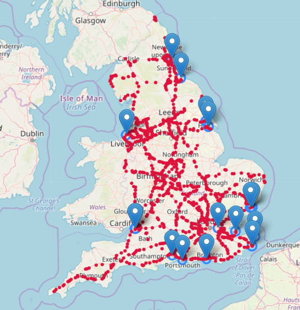
Note that the ports of Avonmouth and Royal Portbury near Bristol have been combined due to their proximity to each other. Felixstowe is combined with Parkeston for the same reason.
Data quality
There are a few data quality issues to consider in this dataset:
- individual sensors can drop out unexpectedly, causing data gaps
- there was a change to the data collection methodology in 2015
- there may be a bias in the positioning of the sensors, which could be preferentially deployed to areas of heavy traffic, and, in recent years, to road sections requiring active traffic management.
Data from individual sensors often has large gaps where no counts are recorded. MIDAS sensors tend to exhibit fewer gaps as they contain a “catch-up” facility where, if the data cannot be transferred immediately due to a network fault or other error, the sensor will store up to eight days of data. They are also directly linked into active traffic management systems so are designed to be more resilient to gaps in the data than TAME or TMU monitoring sites. There are still occasions where no data from a sensor is available for a number of days, weeks or months. This can be caused by software updates, roadworks or where a sensor has failed validation checks. When the latter occurs, the data are not published until the issue is resolved. TAME and TMU sensors do not have a catch-up facility, so there will be gaps for both network and sensor failures. Some of the TAME and TMU sensors are solar-powered and do not function where there is insufficient power available, which also leads to gaps in data collection.
These issues mean that any changes in counts need to be carefully analysed, to ensure any fall in recorded traffic is real and not due to sensor or network failure. The approach we have taken to mitigate potential impact is to aggregate counts over a geographical area, and take the mean value per working sensor in that area. This reduces the overall impact, but at the cost of losing some spatial resolution. For this work this is an acceptable trade-off, as we are interested in overall activity in our geographical locations, rather than behaviour on individual stretches of road.
To analyse the potential impact, we can count the number of observations. There should be one every 15 minutes for each sensor. This allows us to see where there are large changes in the number of observations that may indicate a sensor drop-out. This gives us an indication of the confidence we can place in the measures available. For example, if we observe a large change in traffic figures, but at the same time there is a large change in the total number of observations making up the traffic flow from this period, it implies there is a strong chance that the change in traffic figures is due to a change in the underlying sample rather than a real-world behavioural change.
We do not have available estimates of error in either the counts or speed. However, sensors are subject to regular validation checks administered by Highways England and are taken out of service if they fail. We can have confidence in the accuracy and validity of the data we have acquired. Aggregating the data has the additional benefit of reducing the effect of errors in the counts. For example, if one sensor was over or under counting, but other sensors in the area were working normally, the effect of bias in the data will be mitigated by aggregation.
The count methodology changed in 2015. Between 2007 and December 2014, the traffic between two sensors was counted. From 2015, the counts are collected for each individual sensor. There is also a gap between 31 December 2014 and 1 April 2015 where there is no data, due to the switch over between the old and new systems. Therefore, we require some care in interpreting the time series across the whole period we have data for (2007 to 2018) as differences in traffic flow might be due to a real change and/or might be due to differences in the data collection methodology.
Figure 2: the total number of observations (y-axis) from which data have been collected to construct the indicators
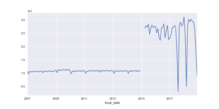
The impact of the change in methodology between December 2014 and April 2015 is clear, as is the gap between those dates. Before the end of December 2014, the numbers represent the number of road sections. From April 2015, they are the number of working sensors
Figure 2 shows the number of observations used to construct the indicators in this paper. The plot clearly shows the impact of the change in methodology between December 2014 and April 2015, and the gap between those time periods. The change in methodology significantly increased the number of observations, but at the cost of increased volatility. Care is required when looking at traffic flow changes for these periods as we do not know if any change is due to changes in the sensors making up these aggregates or a genuine change in traffic flow.
Finally, we expect some bias in the results because, although all major English roads and motorways are covered, sensors may be more densely deployed in areas of heavy traffic, and for active traffic management systems. This means that average speeds – and hence traffic flow – may be dominated by the impact of those systems on traffic flow, and by speed limit decisions, rather than natural traffic flow. This effect is discussed further in Section 3.
Despite these caveats, this dataset is useful to explore as it is large, close to real time, covers the whole of England and is available for granular time periods and geography.
2. Indicator methodology
Tracking the flow of traffic has the potential to provide insights on demand and supply in the UK economy. For example, there is scope to have timelier information on the volume of domestic- and foreign-produced goods that are transported across the UK. It may be that this also offers richer information on regional patterns of activity, which is increasingly of interest to users. Furthermore, it also has the scope to offer some new understandings of the supply potential of the UK, as the analysis of road traffic flows could possibly be used to pick up whether there are disruptions to supply chains in the UK.
Geographic localisation
One area of particular interest in this work is traffic around major ports in England. Timely indication of traffic activity around ports can provide early insight on any potential impact of that activity on the UK economy, which for example may capture the effects of any possible disruptions at the border. Table 1 lists the ports we have included, and Figure 1 maps these together with the road traffic sensor locations.
Table 1: English ports included in this paper. Note that ‘Bristol’ is the sum of Avonmouth and Royal Portbury, due to their proximity to each other. Felixstowe is combined with Parkeston for the same reason.
| Port |
| Bristol – Avonmouth and Royal Portbury |
| Dover |
| Felixstowe and Parkeston |
| Hull |
| Immingham |
| Liverpool |
| London |
| Portsmouth |
| Sheerness |
| Shoreham-by-Sea |
| South Shields |
| Southampton |
| Teesport |
Traffic flow around ports
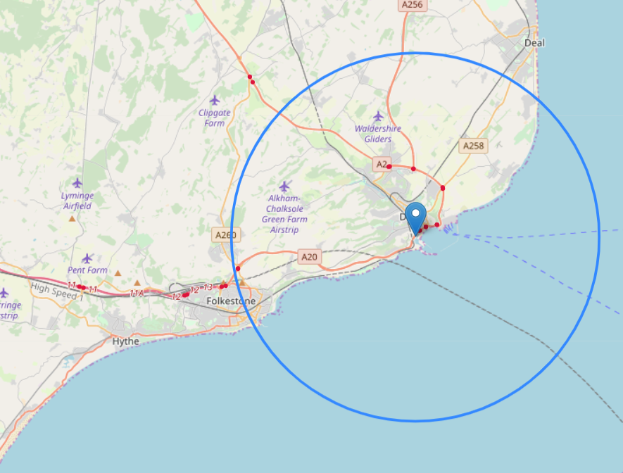
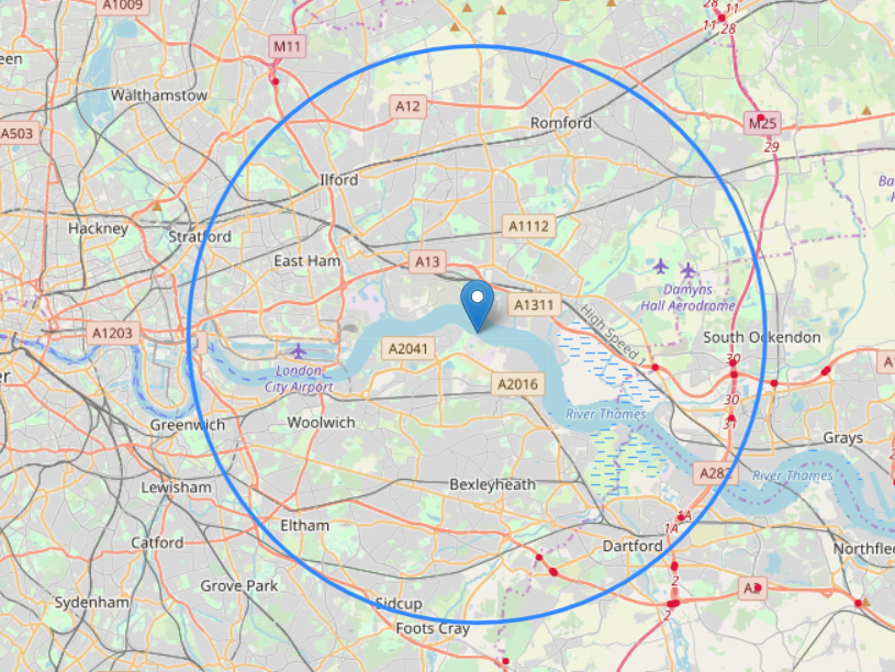
To identify the sensors (2015 to 2018) or road sections (2007 to 2014) to include in the port indicators, we first take the geographic location of each major port in England, using the address and visual inspection. Then we find all sensors and road sections that start or end within a 10 kilometre radius of this point. This means that with the 2007 to 2014 data, due to aggregation in the source traffic counts, we have made sure to include all the data from sensors that are within 10 kilometre of a port. However we will also include data from sensors outside this area, where one of the sensors is within the radius. This means that there is not an exact match between the 2007 to 2014 data and the 2015 to 2018 data, and care must be taken with interpretation. Figure 3 shows the sensors covered for London and Dover.
Figure 3: the sensors (red dots) lying within the blue circles are included in the indicators for Dover (top) and London (bottom)
Traffic flow around ports
There is scope to further refine our methodology for defining port boundaries, using a more complex geometry. While some ports are contained within geographically localised areas, such as Dover, others are spread out over a wider area. The port of London is particularly challenging, as it covers over 50 wharfs spread along a large section of the Thames. An area for potential future work also includes exploring more sophisticated geographies around ports, and obtaining data for Wales and Scotland, which, used in conjunction with traffic direction information, would provide a picture of traffic flows across domestic borders.
Aggregation
Since the data often has gaps in the sensor outputs, we aggregate across each set of sensors or road sections within 10 kilometres of each port, and for all of England. To estimate the average number of traffic counts each month, we:
- sum the total counts in the geographical region, for each 15-minute-interval count from each working sensor
- count the number of observations (each 15-minute-interval count or average speed reading = 1 observation)
- divide the total counts by the number of observations
to give an average count per 15 minutes for each geographical region, per sensor.
To estimate the monthly average speed for each region, we:
- multiply the average speed for each 15-minute observation by the number of counts in each observation in the month
- sum these for all the observations
- sum the total counts contributed from each sensor in the geographical region, for each 15-minute-interval count from each working sensor
- divide by the total number of counts in the observations
to give the average speed over a 15-minute-interval.
By taking an average over all the working sensors, we can mitigate the impact of gaps in the data. The figures presented here should therefore be interpreted as the mean traffic counts per 15-minute-interval, and the mean speed for each month and geography.
Note that, where ports are situated close together, and the 10 kilometre radii overlap, we count each sensor in the overlap region in both port averages. This means that the number of observations across all ports is higher than the total number of sensors, as we are double counting. Future work will investigate the use of improved geographies, and direction of travel information, to refine this approach.
Seasonal adjustment
The monthly series were seasonally adjusted using the standard JDemetra+ seasonal adjustment package, with default settings. Given that there is clearly a break in the series, and the presence of a number of outliers, this approach could potentially be further refined in future work.
3. Results
We compare our monthly indicators of average traffic count and average speed with three official economic statistics:
- monthly gross value added (GVA), chained volume measure (CVM), seasonally adjusted (SA),
- monthly international trade in goods, imports (CVM, SA)
- monthly international trade in goods, exports (CVM, SA)
We make the comparison for the indicators for the all-England traffic flow and for the sum of all the English ports, for all vehicles and for vehicles disaggregated by length.
All-England traffic flow
Figure 4 shows how the average all-England traffic count is affected by the number of observations, that is, the number of sensor readings which contribute to each month’s traffic flow data. It is clear that from April 2015, both the number of observations and the average count is more volatile than previously, and the two troughs in the number of observations in August 2017 and March 2018. These time periods should be interpreted with care. However, the most problematic time period is December 2018, where there is a significant fall in both average counts and number of observations, because data from the MIDAS sensors is currently missing. Therefore it is excluded from further analysis, and we will continue to monitor the situation when we receive the January 2019 estimates.
Figure 4: the all England average traffic counts (right hand axis) and the number of observations (left hand axis)
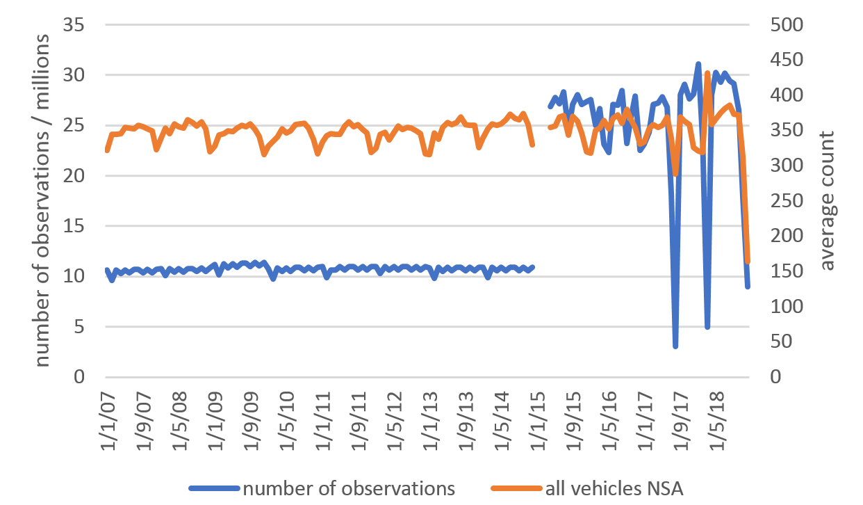
Figure 5 plots seasonally adjusted all-England traffic counts, by vehicle length, against volume estimates of GVA. The counts are dominated by the smallest vehicles, which include cars and motorbikes. Both these series are relatively flat compared with GVA. For the two largest categories of vehicle, the trend follows GVA better, with a prominent fall seen during the last recession. There was also a fall in traffic counts in 2017 and 2018, which is not reflected in GVA, although a fall in UK domestic road freight activity was reported in Domestic Road Freight Statistics, United Kingdom 2017 (Department for Transport). However, we should take some care in interpreting this because there may be data quality issues due to volatility in the number of observations for this period, although, with the notable exception of August 2017, the number of observations broadly rose during 2017.
Figure 5: seasonally adjusted average all England traffic counts, by vehicle length, and GVA (CVM, SA)
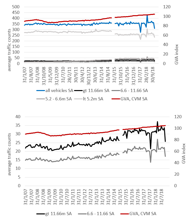
Figure 6 shows the same comparison with international trade in goods
Figure 6: seasonally adjusted average all England traffic counts, by vehicle length, and international trade in goods (imports and exports, CVM, SA)
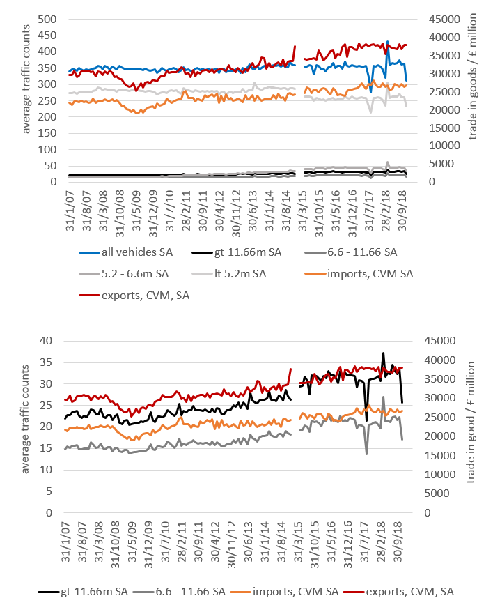
The larger vehicles track imports and exports somewhat better than smaller vehicles. One might expect this to be the case, as international road freight is generally carried out using heavy goods vehicles rather than small cars. However, one might also expect the traffic counts to deviate from international trade estimates, as we make no correction or weighting for the value or volume of goods being transported, as we do not have this information.
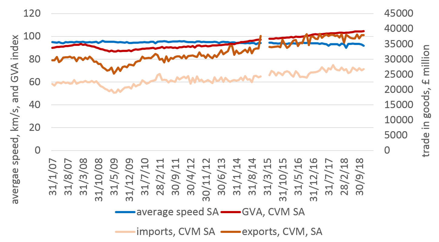
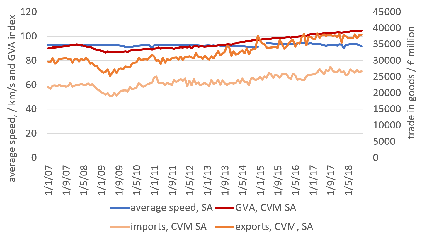
In Figure 7, we show the all England average speed, compared with GVA, imports and exports. There is little relationship between the average speed and the official statistics. Average speed increased slightly in 2008 and 2009, possibly due to a decrease in overall traffic during that period. But in recent years average speeds have fallen, whilst GVA and international trade in goods has risen. Given that traffic counts are fairly level over this period, this could be due to traffic management policies rather than underlying economic effects.
Figure 7: seasonally adjusted average all England speed, km/s, GVA index (CVM, SA) and international trade in goods (imports and exports, CVM, SA)
Traffic flow around English ports
Figure 8 plots the average traffic counts for all the ports with international trade in goods (imports and exports). Once again, we see that traffic is dominated by the smallest vehicle size (cars and motorbikes) and neither the all-vehicle counts, nor the smallest vehicle size fell significantly in value during the recession. For the largest vehicle size, which includes articulated lorries, the picture is somewhat different and a fall in the average counts is seen in 2008 and 2009. There is clearly a break in the series in 2015 and care should be taken in interpreting the rise in average traffic counts between December 2014 and April 2015.
The signal is mixed. Although international freight rose by 5% between 2016 and 2017, to 5.4 billion tonne kilometres (International Road Freight Statistics, United Kingdom, 2017, Department for Transport), domestic road freight fell by 1% to 147 billion tonne kilometres over the same time period (Domestic Road Freight Statistics, United Kingdom 2017 Department for Transport). Given that we – tentatively, given data quality – see a fall in the traffic counts in 2017 for the largest vehicles, which corresponds with domestic road freight statistics, it seems likely that the 10 kilometre zones around ports are picking up domestic freight as well as international. Future work could look more closely at the direction of travel, and access roads to ports, to attempt a better separation of domestic and international freight.
Figure 8: seasonally adjusted average all ports traffic counts, by vehicle length, and international trade in goods (imports and exports, CVM, SA)
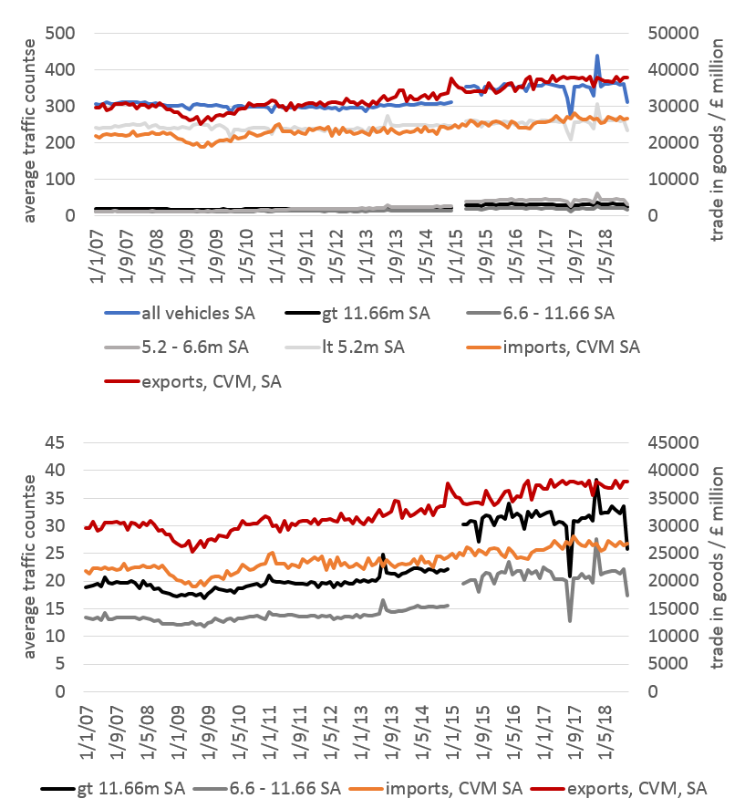
Figure 9 shows the average all-ports speed and again we see a slight rise in average speed during the last recession and falling speed in recent years.
Figure 9: seasonally adjusted all ports average speed, km/s, GVA index (CVM, SA) and international trade in goods (imports and exports, CVM, SA)
4. Conclusions and future work
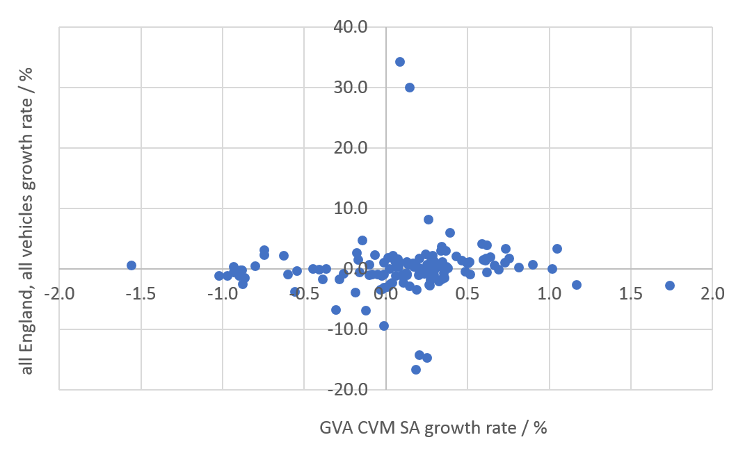
Tracking the flow of traffic has the potential to provide insights on demand and supply in the UK economy. We conclude that the road traffic counts give us some interesting insights into road transport in England, although they require careful interpretation. In particular, there is some evidence that traffic counts for the largest vehicles are consistent with at least some economic events, such as the last recession. We anticipate that these indicators will be used to understand traffic movements, and perhaps for early indications of large economic changes where movement of goods or people is important. We do not recommend using the indicators to predict GDP or other headline economic statistics on their own. As we see in Figure 10, there is not a strong relationship between road traffic count and GVA growth rates, and there is a large scatter.
Figure 10: all England average traffic counts for all vehicles (SA) and GVA (CVM, SA), growth rates, showing a large scatter in the relationship
Further work is required to improve how understanding of how this can be used a faster indicator of economic activity, specifically, how traffic by different types of vehicles relate to local, national and international economic activity involving the transport of goods and people. This will help in identifying the extent to which this can be used to inform users of how effects in the domestic and global economy might be reflected in these timely indicators.
We publish our historical estimates with this work. The full datasets, including breakdowns by port, can be found in the Faster indicators of UK economic activity: dataset. We propose publishing monthly road traffic indicators with a two-month lag (for example, publishing indicators for February in April). We hope to be able to access the data faster in future, to reduce the lag to one month. The first publication is planned for mid-April 2019, with an article setting out the full set of faster indicators of UK economic activity (including those based on VAT returns and shipping) and the format of the publication to be released in advance.
Having completed this initial exploration of the data, and made these time series available on a regular basis, potential future areas for exploration include:
- accessing similar information for Wales, Scotland and Northern Ireland, and including analysis of cross-border traffic, using information on direction of travel
- developing interactive maps and visualisations, to allow users to explore this rich dataset in more detail, and linking these to our new shipping indicators by port, as a potential indicator of how quickly goods are moved around the country
- improving the geographical bounding boxes around the ports, and incorporating information on direction of travel, to investigate whether international road freight can be better isolated from other types of road use
- analysis of the traffic for additional geographies, such as around geographical areas with high production or warehousing activity, this might be of particular interest in understanding just-in-time supply chains
- further breakdowns of the indicators, for example, by time of day, day of the week, averages over shorter time periods – although care will need to be taken with data quality
- exploring whether road traffic counts might be lagged or leading indicators for official economic statistics
- comparing the traffic counts with other economic indicators, for example, household consumption, or employment.
We welcome feedback on this work, which can be sent to faster.indicators@ons.gov.uk.
5. Authors
Edward Rowland, Arturas Eidukas, Stephen Campbell, Louisa Nolan, Duncan Elliot, Sumit Del-Chowdhury