Data science for the public good

Project summary

Many datasets contain variables that have been collected as free-text in an uncontrolled way. In the case where this information contains items or short textual descriptions the goal is to aggregate similar entries to analyse the quantities of these that appear within the dataset. This textual information usually requires a significant amount of manual processing which can be impractical for large datasets. The Data Science Campus have developed a processing pipeline which can automatically group and generate hierarchical labels for each group to structure the data. We have written this blog to introduce the pipeline which can be found in our optimus Github repository.

Introduction

In the current political climate there is much interest in understanding and measuring the volume and type of goods travelling through UK ports. The Data Science Campus are working with the Department for Environment, Food and Rural Affairs (DEFRA) to analyse manifest data collated by ferry operators to understand port-level trade flows. This project aims to apply modern techniques of natural language processing (NLP) to process these datasets automatically and generate a classification of the type of goods being transported, so that groups of similar product types and their flows can be analysed.

The goal of the project is to create a hierarchical classification of the goods being transported. Here, we detail our initial work and the processing pipeline we have created. So far we have developed a pipeline that takes text descriptions of lorry level contents and returns this original dataset with an extra variable which is the automatically generated label for the type of contents contained.

Processing free-form text

More on the data source

Ferry operators collect information on the contents of lorries and trade vehicles boarding their vessels. The data is collected in an uncontrolled manner and no previous analysis of the free-form text collection has been possible due to complexity and skills required to process the data. This means that, for each vehicle, a single-line description of the contents of the vehicle, as reported by the driver, is recorded. As there are no controls on how this data is collected, the operative may write their own interpretation of the contents complete with their own personal shorthand – for example, they may use “MT” or “M/T” or both in different instances, as a code for signifying an empty vehicle – before this data is later collected and digitised.

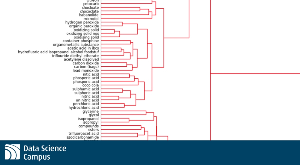
Experienced analysts may expect two levels of human input to lead to typos and other errors and this is indeed the case. We see many instances of “chococolate”, “chococlate” and “chocolate” just to keep us on our toes. The first stage of our processing was to identify how we deal with these kinds of issues and the level to which we need to pre-process the data source. For this first phase of the project we actually took a pretty light touch as our pipeline handled many of the mis-spelt words and let us deal with deeper methodological concerns instead of building a bespoke spell-checker for ferry data!

Generating numerical representations of item descriptions

The main aim of this project is to obtain a clustering of text descriptions that capture the contextual relationship between item descriptions. To do this we need to convert each text description into an appropriate number so that we can perform meaningful clustering on the values that items correspond to. To do this we made use of a pretrained word embedding model, Facebook’s FastText tool. This was chosen because it not only takes into account the spelling of words but also those words that are commonly used in conjunction with it. FastText uses the English language Wikipedia content to model the word relationships to generate context aware numeric embeddings in 300 dimensions. It is FastText that allows us to bypass the spell-checking mentioned above as it can handle embedding words it has never seen before.

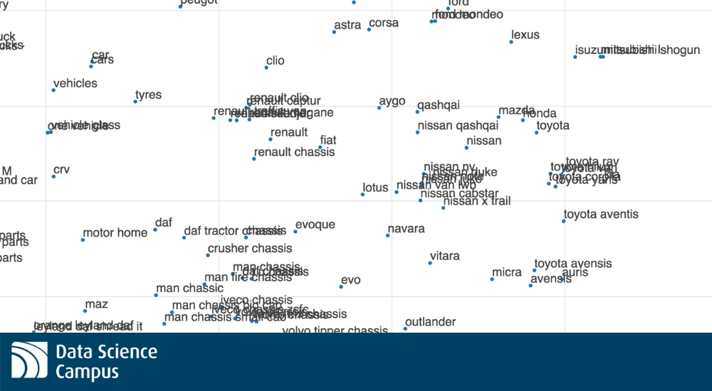
Here is an example visualisation of the embedding – as you can see we have a clear cluster containing a large number of chemicals. Similar groupings are found across the whole space and we find that the clusters we obtain generally make quite a lot of sense.

Our first pass at this was more successful than we would have expected for a naive attempt with little pre-processing of the data. However, it was not without its problems. For example, we found that descriptions containing the word “products” such as “steel products”, “paper products” were all clustered together. What we would prefer is if the “steel products” description was instead in a cluster with all of the steel items so as to provide more suitable clusters further down the line. This was implemented by encoding the word “products” as “P” so that it carries less weight in the embedding because of its new shorter length. A list of encodings was created to handle words in this way if we felt that they did not add value to the type of item being considered. This simple step moved a lot of items around and significantly improved the quality of the embeddings.

From here we were able to perform our clustering on the embedded vectors using Ward linkage so as to generate clusters ready for relabelling.

Generating cluster labels

Once the clusters were identified we needed to decide programatically how to take their contents and generate a suitable replacement label for those items. With clusters generated not just on similarity of spelling of the item descriptions but also on the context of words, we developed a series of evaluations and subsequently a way of relabelling clusters to fit this approach.

The method begins by identifying clusters of items formed that are similar in terms of the numeric value obtained through the embedding. This way we can first consider the items that are most closely clustered, and work outward. Each cluster is sequentially evaluated against four classifiers that start by considering syntactic similarity and progresses through less strict comparisons, until we land at the stage considering semantic similarity of the words in the cluster. Each classifier has a distinct protocol for relabelling the cluster:

Edit distance comparison

The Levenshtein distance is a metric that determines the minimum number of character level changes that need to be made to get from one word to another. For example, if you wish to change the word “cat” into “crash” then we must make the following changes: i. insert the letter “r” into “cat” so we get “crat” ii. insert the letter “h” at the end of “crat” to get “crath” iii. replace the letter “t” with an “s” and we get to our desired “crash” This is the shortest way in which to turn “cat” into “crash” and so we say that the edit distance, which is synonymous with Levenshtein distance, is 3.

If the average Levenshtein distance between all of the possible pairs of descriptions in the cluster was lower than some chosen threshold then we assign the most common description to the label for the cluster.

Common words comparison

We built functionality to compare strings for sets of common words within each cluster and where these common words passed a certain condition they were selected as the new label. For example, if we had the three descriptions “aluminium cages”, “aluminium tubes”, “aluminum sheets” then we may allow the use of “aluminium” to replace all of these.

Common substring comparison

This is the same as in 2, but we searched for common substrings, so where we only consider whole words above this we can match cases where only parts of words are similar.

WordNet lookup

At this point we have exhausted our syntactics comparitors and so we use WordNet to look up the higher-level meanings of the words in the cluster and use a suitable common root word as the label. For example, “apples” and “oranges” would have “edible fruit” as a common parent and so it is what we use.

Of course, there are instances where none of these tests result in a suitable label being applied for a cluster. If this is the case, these unlabelled items are placed back into consideration along with the new labels replacing old item descriptions. The process is then repeated but the distance at which clusters are allowed to form is increased so that each iteration of the pipeline can develop a more general label for a larger cluster. You may think of this as each of the clusters we originally form being allowed to absorb more of the things around them to create a more generalised label for the things that the cluster represents.

Where we are now

We have now built a program to perform all of the above and have repeated the process to generate class labels for over 80% of the test dataset. The next stage is to work with DEFRA to evaluate the performance of the pipeline and apply this to other datasets, which will allow us to refine the methodology.

Our results so far are promising. The embedding has worked as intended and we clearly see clusters of items that contain almost all of the cars transported; but even within this we see subclusters where many of the French makes are grouped with each other and similarly for the Japanese car brands such as Nissan and Toyota.

We have released code for optimus on our github.com repository. In the future we aim to generalise the product into a tool that you can put any kind of product dataset into and create a clustering and classification of the items it contains. We are also intending to use the labelled datasets we obtain to train a supervised model to project our labels onto a more widely used classification system such as the Trade Tariff codes used by HM Revenue and Customs.

Caveats

We close with a few words on some of the main issues we will face in making this tool more widely used and available. The largest issue will always be the need for manual recalibration of some of the labels and sense checking of what the algorithm spits out. However, given that the data is currently almost unusable and we are able to reduce the burden on those people interested in unlabelled free-text data by some orders of magnitude, we are content with this.

This phase of the project does not allow us to measure volumes of any specific good being transported – just instances – and so for the ferry data our unit is “lorry carrying some quantity of…”. It is quite common that this isn’t available in the data, and is therefore not possible to attempt, but this should be taken into consideration for those interested in weights and quantities of items.

Finally, it will be difficult to verify the quality of the final output and we are currently relying on manual inspection to evaluate the noise. We are beginning to think about how the data can be quality assured to some extent.

Thanks for reading. If you would like any more information please contact the Data Science Campus.