Technical report: Estimation of travel to work matrices

Travel to work matrices show movement of people from their home location (origin) to their place of work (destination) at an aggregated level. The Office for National Statistics (ONS) collects travel to work data from the census every 10 years, with the most recent being 2021. This travel to work data allows the generation of travel to work matrices for census years, for instance, at 10-year intervals with no updates for years in-between.
Using aggregate spatial modelling approaches, we have produced an alternative estimation of the travel to work matrices which bridges this gap. We have produced experimental data for each year from 2012 to 2021 and have published modelled estimates for 2021. When new data becomes available, the model can also estimate the travel to work matrices from 2022 onwards. For 2021, the model provides travel to work estimation assuming pre- and mid-coronavirus (COVID-19) pandemic commuting behaviours, respectively. This will provide complementary statistics to the Census 2021 travel to work data collected during the pandemic, which is affected by pandemic travel patterns. These modelled estimates are the first release in a planned work programme of incremental improvements to the model and outputs. Please note that these are the experimental results and should not be used for decision making purposes. We welcome feedback via datasciencecampus@ons.gov.uk.
Using the Census 2011 travel to work data as ground truth, we employed doubly constrained gravity approach, for our initial travel to work estimation, to calibrate the base year model. The calibrated model is then used to estimate the travel matrices between homes and fixed workplaces for all future years (i.e. 2012 to 2021). For future year estimation, the model requires, as input, the total working population at residential zones and total employees at workplace zones.
To this end, various data is used to estimate growth rates (reference to the base year of 2011) of resident workers with fixed workplaces at origin zones (residential end) and number of employees at destination zones (workplace end). We use the National Travel Survey (NTS and the National Trip Ends Model (NTEM) to estimate changes in working population at residential end and employees at workplace end for all future years. For 2021, we additionally used Census 2021 (instead of NTEM used for 2012 to 2020) for more accurate estimate of growth in total population at residential end. Then an iterative process, called the doubly constrained model is applied to assign the numbers to the travel to work matrix ensuring that estimated number of resident workers at all origins matches the number of employees working at all destinations. Doubly constrained models ensure matching the totals at both residential and workplace end of travel to work matrices.
We have investigated the data quality of these input data, which demonstrate in some occasions low confidence at fine spatial granularity because of their sample size, response rate and coverage. This will affect the spatial granularity and reliability of the results the model can estimate. Another shortcoming of the estimated travel to work matrices is the lack of validation, which has not been possible in the absence of a representative survey of travel to work for 2021, for example, the context of Census 2021 previously discussed.
In response to the aforementioned shortcomings, in our future work, we are considering use of additional or alternative data sources to improve the model and to validate the outputs. These include:
- mobility data, such as aggregated footfall data derived from mobile phone users
- Labour Force Survey (LFS)
- Business Register and Employment Survey (BRES)
- working with teams within the ONS to specify fused datasets, for instance, linking address and business indexes to estimate populations within areas grouped by occupation and industry types
Alongside exploring other data sources, we also plan to apply further improvements in our modelling approach, including segmentation by important socioeconomic and demographic groups (who tend to adopt different commuting behaviours) and facilitating scenario–based analysis for agile decision making. This allows accounting for uncertainties in future economic, social, and technological evolvements which can affect travel to work such as growth in the rates of working from home or hybrid working in some industrial sectors and job types, or emergence of new technologies like autonomous vehicles.
Table of contents
1. Introduction and background
Travel to work (TTW) matrices show movement of people from their home location (origin) to their place of work (destination) at an aggregated level. Information on travel to work informs both national and local transport services and policies. It provides a basis for transport planning, for example, whether new public transport routes or changes to existing routes are needed. Additionally, it allows the measurement of environmental impacts of commuting, such as traffic congestion and pollution, and how these might change over time, for example because of changes in commuting modes, such as a shift from car to bicycle.
The Office for National Statistics (ONS) collects travel to work data from the census every 10 years, with the most recent being 2021. This travel to work data helps us generate travel to work matrices for census years, for instance, at 10-year intervals with no updates for years in-between.
Census 2021 was undertaken during a period of rapid change, during the coronavirus (COVID-19) pandemic. Government guidance was to stay at home where possible and avoid public transport. There was a shift to home working for those in industries and occupations that could, and approximately 5.6 million jobs in England and Wales were supported by the furlough scheme around the time of Census 2021.
This means that travel to work data from Census 2021 is a combination of pre- and mid-pandemic travel behaviours, and it is unclear how furloughed respondents answered census questions. Changes such as hybrid and home working may be here to stay, but there will also be some return to pre-pandemic travel behaviours. It is therefore unclear how representative and useful Census 2021 TTW data is to policy makers given the context. More information is available on the quality of the travel to work census data.
Other sources of travel data are available, such as the National Travel Survey (NTS) produced by Department for Transport (DfT), or travel to work modules in the Opinions and Lifestyle Survey (OPN). However, neither source provides comprehensive travel to work matrices or reliable data below regional level, which is important for travel planning. For this reason, ONS is embarking on research to understand where novel modelling methods could be used to improve the timeliness and resolution of travel to work estimates.
Using aggregate spatial modelling approaches, the Data Science Campus has produced an alternative estimation of the travel to work matrices which bridges this gap. We have produced experimental data for each year from 2012 to 2021 and have published modelled estimates for 2021. When new data becomes available, the model can be updated to include 2022 onwards.
This will provide complementary statistics to the Census 2021 travel to work data collected during the pandemic, which contains a mixture of pandemic and pre-pandemic behaviours by estimating, for example, separate travel to work matrices using both pre– and mid-pandemic commuting behaviour. These modelled estimates for 2021 are the first release in a planned work programme of incremental improvements to the model and outputs.
We have developed a detailed roadmap, this report and resulting experimental data are the first stage in this road map and are published to compliment the Census 2021 travel to work data, and to gather feedback from stakeholders on the technical specification and outputs. The technical specification of the gravity model is provided in Section 3 with the summary of input data provided in Section 2. Initial results are shown in Section 4. We discuss and conclude our methodology in Section 5 and 6, respectively. A broad summary of future stages to build on the current gravity model and to move towards a scenario-based recursive spatial equilibrium model in our vision is provided in Section 7.
2. Data
The input datasets used in the first release of the gravity model are listed in Table 1.
Table 1: List of the data sources used in the latest pipeline of the gravity model
| Dataset Name | description | Data owner |
| wf02ew_oa | Census 2011 travel to work matrix, England and Wales | ONS |
| TS066_Economic_activity_status | Census 2021 employment status table | ONS |
| core_planning_growth_factor_v8 | National Trip End Model (NTEM) v8 core scenario planning data 2011 to 2021.
The National Trip End Model forecasts the growth in trip origin and destination up to 2051 for use in transport modelling. The Core_planning growth_factors_v8 dataset includes the growth of employment and population up to 2051. |
DfT
https://www.data.gov.uk/dataset/11bc7aaf-ddf6-4133-a91d-84e6f20a663e/national-trip-end-model-ntem
|
| Various ONS Geography tables | Census 2011 definitions
Census 2021 definitions Lookup tables between Census11 and 21 definitions Census 2011 Population Weighted Centroids |
ONS
https://geoportal.statistics.gov.uk/
|
| national_travel_survey.household and inidividual
|
National Travel Survey (NTS) 2011-2021 household and individual tables.
NTS is a household survey designed to monitor long-term trends in personal travel which collects information on how, why, when and where people travel as well as factors affecting travel by residents of England. |
DfT
https://www.gov.uk/government/collections/national-travel-survey-statistics |
| Latent geographic clusters | Land use and travel clusters defined by land use characteristics including area type, population density and accessibility measures – this is derived based on NTS data; the methodology is reported in Jahanshahi & Jin (2021). | Jahanshahi and Jin |
As this work is incremental to improve the modelling and output quality with more data sources, we plan to add several datasets to this framework, including Labour Force Survey (LFS), Business Register and Employment Survey (BRES) and mobile phone data. For more details, please refer to Section 7: Future steps.
3. Methods
The work described in this section builds on a framework of the classical gravity model described in chapter four and five, Modelling Transport which includes production and attraction estimation, calibration of the deterrence (cost) function and doubly constrained modelling. We have redefined and extended the classical gravity model as below:
- redefine the terminology used in the classical gravity model to accommodate our research question to follow the census travel to work definitions (see section on formalising the research question in the gravity model)
- combine various data sources shown in Table 1 and the use of latent geographic cluster analysis (see Appendix C) to estimate the production and attraction (see section on the Production and attraction estimation module) in future years, that is, the total population aged 16 years and over who are in employment and travel to a fixed workplace (at residential end), and the number of employees attracted to workplaces (at workplace end)
- use the curve fitting method to improve the calibration of the deterrence (cost) function instead of the classical Hyman’s method (see section on Calibration of the cost function )
This section starts with an introduction to the gravity model; we formalise the research question and then show the processing pipeline and details of each module including the production and attraction estimation, calibration of the cost function and doubly constrained model.
Introduction to the gravity model
Equation (1) shows a simple form of gravity model which is an analogy of Newton’s gravitational law. \( \)
\(T_{ij}=(α*P_i*P_j)/(d_{ij}^2) \) (1)
Where \(T_{ij}\) is the number of trips between zones i (origin) and j (destination), \(P_i\) and \(P_j\) are the populations of the origin i and destination j, \(d_{ij}\) is the distance between i and j, and α is a proportionality factor.
This was further generalised and improved to the following classical format shown in Equation (2).
\(T_{ij}=A_i*O_i*B_j*D_j*f(c_{ij}) \) (2)
Where \(A_i\) and \(B_j\) are balancing factors, \(O_i\) and \(D_j\) are the trip ends, cij is the cost (either travel deterrence elements or combination of those such as travel time, cost, and distance) to travel between i and j. For this first version of model, we used travel distance as the deterrence element. \(f\left(c_{ij}\right)\) is the cost function, often received as ”deterrence function” because it represents the disincentive to travel as distance or cost increases. Some popular cost functions are:
\(f(c_{ij} )=exp(-β*c_{ij}) \) (3)
\(f(c_{ij})=c_{ij}^{-n}\) (4)
\(f(c_{ij})=c_{ij}^n*exp( -β*c_{ij}) \) (5)
The trip end generation of \(O_i\) and \(D_j\) is described in the processing pipeline section. The parameters (such as β, n) in the cost function should be estimated in the calibration process which is described later. \(A_i\) and \(B_j\) can be calculated via an iterative process for a doubly constrained model.
Formalise the research question in the gravity model
We follow the census travel to work definition, which is different from the traditional terms and definitions used in transport modelling, particularly in modelling trips or tours. The census travel to work dataset provides the commuting flow between the area of residence and area of workplace, aggregated to census geography, such as MSOAs of the usual residents of England and Wales aged 16 years and over and in employment. For example, the 2011 Census travel to work (TTW) table is generated from 2011 Census Questionnaire 40 shown in Figure 1. Those with no fixed place of work, those working at or from home and those working offshore are included as special non-geographical destinations (OD0000001 = Mainly work at or from home, OD0000002 = Offshore installation, OD0000003 = No fixed place, OD0000004 = Outside UK) in the census TTW dataset but not in our estimated travel to work matrices. Our estimated dataset provides commuting flow for those with a fixed workplace, that is, the location of people’s main job. Traditional transport models, such as the gravity model, normally provide the number of trips and often some temporal element, such as whether trips occur during peak or off-peak times. The census questions do not include the number of trips or time of trip, but usual residents’ home address and the address of their workplace for their main job. For example, the 2011 Census TTW statistics do not provide the trip statistics during peak or off-peak time or day of week. If the trip rates in a certain period of time (for example, daily or weekly) is known, the number of people provided in census can be converted to number of trips by multiplying census outcomes by trip rates.
Figure 1: Census 2011 Question 40

To formalise our research question, estimate the TTW matrix using the gravity model, we define the meaning of components in Equation (2).
Working population: the number of people aged 16 years and over who are in employment.
\(T_{ij}\) is the number of people aged 16 years and over who are in employment living at area i and travelling to a fixed workplace j; to avoid T being confused with time, \({OD}_{i,j}\) is used to replace \(T_{ij}\) in the rest part of this document.
\(O_i\) (called production) is the number of the working population who live at area i and travel to a fixed workplace.
\(D_j\) (called attraction) is the number of employees working at a fixed workplace j.
\(A_i\) and \(B_j\) are balancing factors and are calculated during iterative procedure in a doubly constrained model.
In the current version of the gravity model, the spatial granularity (i and j) is 7201 MSOAs covering England and Wales following the 2011 Census geographical definition.
b is the base year as the ground truth. In the current version, we use Census 2011 TTW dataset as the base year’s data.
t is the future year.
Figure 2: The base year TTW matrix and the expected Oi and Dj at the future year t
| Destination (D) | |||||||||
| MSOA0 | MSOA1 | … | MSOA j | … | MSOA N-1 | \(O_i^b={\sum_{j=0}^{N-1}}OD_{ij}^b\) | Target
\(O_i^t\) |
||
| Origin
(O) |
MSOA0 | \(OD_{0,0}^b\) | \(OD_{0,1}^b\) | … | \(OD_{0,j}^b\) | … | \(OD_{0,N-1}^b\) | \(O_0^b\) | \(O_0^t\) |
| MSOA1 | \(OD_{1,0}^b\) | \(OD_{1,1}^b\) | \(OD_{1,j}^b\) | … | \(OD_{1,N-1}^b\) | \(O_1^b\) | \(O_1^t\) | ||
| … | … | … | … | … | … | … | … | … | |
| MSOAi | \(OD_{i,0}^b\) | \(OD_{i,1}^b\) | … | \(OD_{i,j}^b\) | … | \(OD_{i,N-1}^b\) | \(O_1^b\) | \(O_i^t\) | |
| … | … | … | … | … | … | … | … | … | |
| MSOAN-1 | \(OD_{N-1,0}^b\) | \(OD_{N-1,1}^b\) | … | \(OD_{N-1,j}^b\) | … | \(OD_{N-1,n-1}^b\) | \(O_{N-1}^b\) | \(O_{N-1}^t\) | |
| \(D_j^b={\sum_{i=0}^{N-1}}OD_{ij}^b\) | \(D_0^b\) | \(D_1^b\) | … | \(D_j^b\) | \(D_{N-1}^b\) | ||||
| Target
Dtj |
\(D_0^t\) | \(D_1^t\) | \(D_j^t\) | \(D_{N-1}^t\) | |||||
Figure 3: The cost matrix
| Destination (D) | |||||||
| MSOA0 | MSOA1 | … | MSOA | … | MSOAN-1 | ||
| Origin
(O) |
MSOA0 | c0,0 | c0,1 | … | c0,j | … | c0,N-1 |
| MSOA1 | c1,0 | c1,1 | c1,j | … | c1,N-1 | ||
| … | … | … | … | … | … | … | |
| MSOAi | ci,0 | ci,1 | … | ci,j | … | ci,N-1 | |
| … | … | … | … | … | … | … | |
| MSOAN-1 | cN-1,0 | cN-1,1 | … | cN-1,j | … | cN-1,N-1 | |
In Figure 2, the base year TTW matrix (2011 Census TTW matrix, \({OD}_{i,j}^b\)) is the white area, and the grey columns and rows are the expected production \(O_i\) and \(D_j\) attraction for the future year t (generated from the production and attraction estimation module; in our model, we are dealing with number of people rather than trips). Figure 3 is the cost matrix which can be generated from the census travel to work statistics, for example, to estimate a matrix of travel distance, or other deterrence elements such as travel time and cost. We use the base year 2011 Census TTW matrix combined with other geographical data to calculate a population weighted centroid travel distance matrix between MSOAs (see Appendix A) as the cost matrix, and then to calibrate the cost function (Equation (5)). The calibrated model in the base year is then used (using Equation (2)) to estimate future year TTW matrices, \({OD}_{i,j}^t\) where the grey cells in Figure 2 are input \(O_i^t\) and \(D_j^t\) in Equation (2).
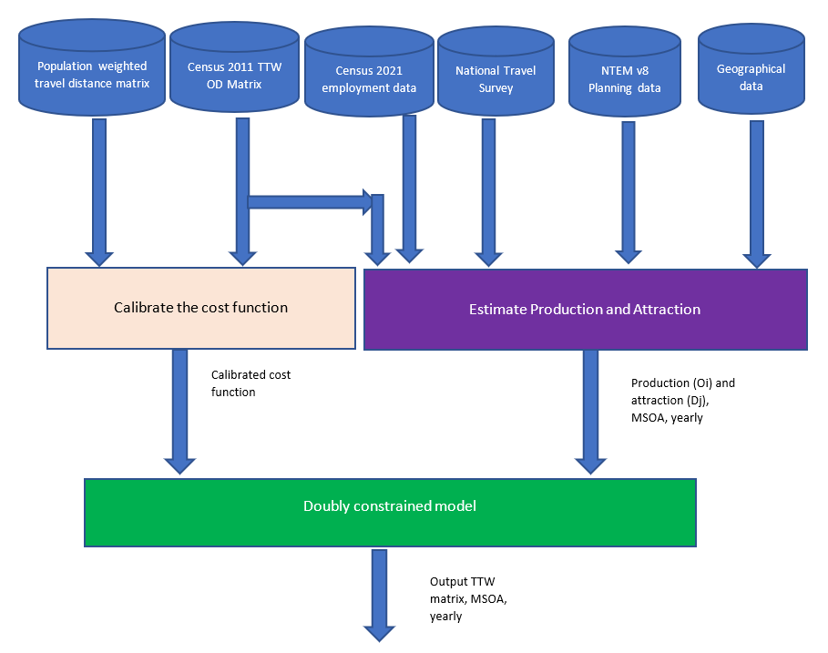
Processing pipeline
Figure 4 shows the processing pipeline which includes three core modules:
- estimation of production and attraction module: to estimate \(O_i\) and \(D_j\)
- calibration of the cost function: to calibrate \(f\left(c_{ij}\right)\)
- doubly constrained module: to estimate \(A_i\) and \(B_j\)
The 2011 Census TTW matrix and the population weighted distance matrix (the cost matrix) are used to calibrate the cost function in the base year. Oi and Dj are estimated using various data sources to estimate the production (\(O_i\)) and the attraction (\(D_j\)) in future years. In our model we will simply call this production and attraction module as we are not dealing with trips for TTW matrices (refer to Section 3.2. for definitions). In the latest version of the gravity model, 2011 Census TTW matrix, Census 2021 employment data, NTS, NTEM v8 core scenario planning data and latent geographic clusters (based on Jahanshahi and Jin are fused to estimate \(O_i\) and \(D_j\) for all future years. The doubly constrained model will calculate\(A_i\) and \(B_j\) via an iterative process (doubly constrained module) and finally output the TTW matrix for the future year.
Figure 4: The processing pipeline of the gravity model
Production and attraction estimation module
The production and attraction estimation aims at estimating or predicting the total number of the working population who travel to a fixed workplace (production \(O_i\)) as well as the total number of employees attracted to a workplace (attraction \(D_j\)). The calculation is decided by the availability of data sets, their granularity and quality. A brief description of the calculation procedure is as below. For more details refer to Appendix B and C.
Estimation of production Oi
Production \(O_i\) is the number of the working population who travel to a fixed workplace. The Census 2021 was undertaken during the coronavirus (COVID-19) pandemic, when government guidance was to stay at home where possible and avoid public transport. There was a shift to home working for those in industries that could, and up to 5.6 million jobs were furloughed in those industries that could not. Census 2021 employment dataset reports the employment status of the population in England and Wales as a snapshot in time. The guidance on Census 2021 says that the respondents should answer the travel to work questions based on their situation immediately before the current period away from work, however, it is not clear whether the working population under the lockdown and furlough policy followed the revised guidance precisely. More information on the quality of the Travel to Work Census Data is provided in which indicates that travel to work data is a combination of pre- and mid-pandemic travel behaviours.
The Census 2021 release currently includes statistics on the working population, distance travelled to work, method used to travel to work but not the travel to work matrices. The Census 2021 reports that in England and Wales, 15.1 million people travel to a workplace or depot (54.3% the working population). The 2011 Census reports that in England and Wales, 21.6 million people travelled to a workplace or depot (81.0% the working population). This comparison shows a significant drop of 26.7 percentage points in the working population commuting to a main workplace or depot from 2011 Census to 2021. It indicates the influence of the pandemic on Census 2021 travel to work responses. Therefore, the Census 2021 travel to work data cannot reflect the pre- or post-pandemic population commuting patterns. Thus, we do not use the Census 2021 travel to work data, neither the working population in the fixed place of work (\(D_j\)) from Census 2021.
Instead, for estimation of the production in 2021, we used the total working population from Census 2021 and estimate the proportion of those who work at fixed places from the National Travel Survey (NTS) data. To account for spatial variations of travel patterns, separate estimation of working at fixed places is generated for each latent geographical cluster. Latent geographical cluster is estimated based on land use and area characteristics such as area type, population density and accessibility measures; the clusters are proved to have close association with travel patterns and behaviour.
These are the steps to calculate \(O_i\):
- Step 1. Get the working population, \({workingpop}_i^t\) at MSOA i, England and Wales from Census 2021 employment dataset, where t=2021. Please note that for the Census 2021, some MSOA definitions have changed when compared with Census 2011; some MSOAs are merged and some others are split. We generate a lookup table from MSOA21 to MSOA11 definition for consistency. Annex B shows more details on the lookup table and translation between MSOA21 and MSOA11. For other years between 2011 to 2021 (2012 to 2020), we use NTEM v8 (core scenario) growth factors of the working population \(g_i^t\) to calculate the working population.
\({workingpop}_i^t={workingpop}_i^b\ast g_i^t\)
Where \({workingpop}_i^b \) is the working population from 2011 Census, 2012 ≤ t ≤ 2020.
- Step 2. Estimate the ratio (\(r_i^t\)) of the working population travelling to a fixed workplace using NTS and latent geographic cluster analysis for each MSOA. This assumes that all the MSOAs within the same cluster share the same growth rate. This ratio can be aggregated from NTS 2018 to 2019 to reflect the pre-pandemic commuting pattern or from NTS 2020 to 2021 to reflect the influence of the pandemic to commuting patterns. As NTS is an annual survey, \(r_i^t\) can be updated yearly. For more details, refer to Annex C.
- Step 3. Calculate \(O_i^t\).
\(O_i^t=r_i^t\ast{workingpop}_i^t\)
Where \(r_i^t\) is calculated in Step 2 and the same growth rate is applied to all MSOAs in each cluster.
Estimation of attraction \(D_j^t\)
Attraction \(D_j^t\) is the number of employees in a fixed workplace j. The ”jobs” from NTEM v8 (core scenario) planning data is used as the proxy for total employment available within each MSOA. This is different from the census TTW matrix definition where \(D_j\) is the number of employees attracted to a fixed workplace. Assuming the number of jobs is highly correlated with the number of employees working at that zone as a fixed workplace, \(D_j\) is calculated using jobs growth factor from NTEM v8 core scenario planning data.
As Census 2021 has not published the number of employees at local areas at the time of publication of this report, 2011 Census data is used as the ground truth \(D_j^b\).
\(D_j^t=D_j^b*g_j^t\)
Where \(D_j^b\) is the number of employees working at MSOA j as fixed workplaces from 2011 Census.
Where \(g_j^t\) is the ”jobs” growth factor from the base year 2011 to the future year t at MSOA j.
Please note that NTEMP forecasts are subject to uncertainty, especially when disaggregated to local zones; for example, growth factors at the MSOA level have low confidence. We plan to cooperate with DfT to improve this in the future versions. We are also exploring alternative data sources for estimating employment growth by type of jobs and industries.
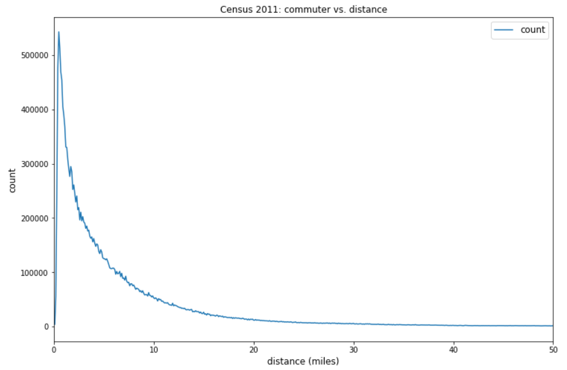
Calibration of the cost function
We calibrate the model against Census 2021 TTW data (the ground truth). In calibration, we evaluate the best cost function form to employ \(f\left(c_{ij}\right)\) and then estimate the parameters in the cost function to achieve the best match to the commuting profile in the observed data (i.e. Census 2011).
In our current model, considering the data availability, we chose the travel distance as Annex A introduces more details on the method of population weighted centroid travel distance. We have also decided to use combined function as \(f\left(c_{ij}\right)\). Figure 5 shows the distribution of the commuting distance based on Census 2011 travel to work data where the number of commuters increases in short distance and then drops sharply at medium/long distance. Thus, the combined function \(f\left(c_{ij}\right)={k\ast c}_{ij}^n\ast\exp{\left(-\beta\ast c_{ij}\right)}\) is chosen as the best cost function form to replicate this observation. Three parameters (k, n and b) are calibrated using the curve fitting method: b=0.306, k=0.0217, n=0.231.
Figure 5: 2011 Census distribution of travel distance, England and Wales
The calibrated cost function demonstrates some difference from the base year, particularly for short-medium commuting distance. Figure 6 shows the travel distance distribution between 2011 Census and the calibrated model where discrepancy is smaller for the longer travel distances.
Figure 6: 2011 Census travel to work distance comparison, England and Wales
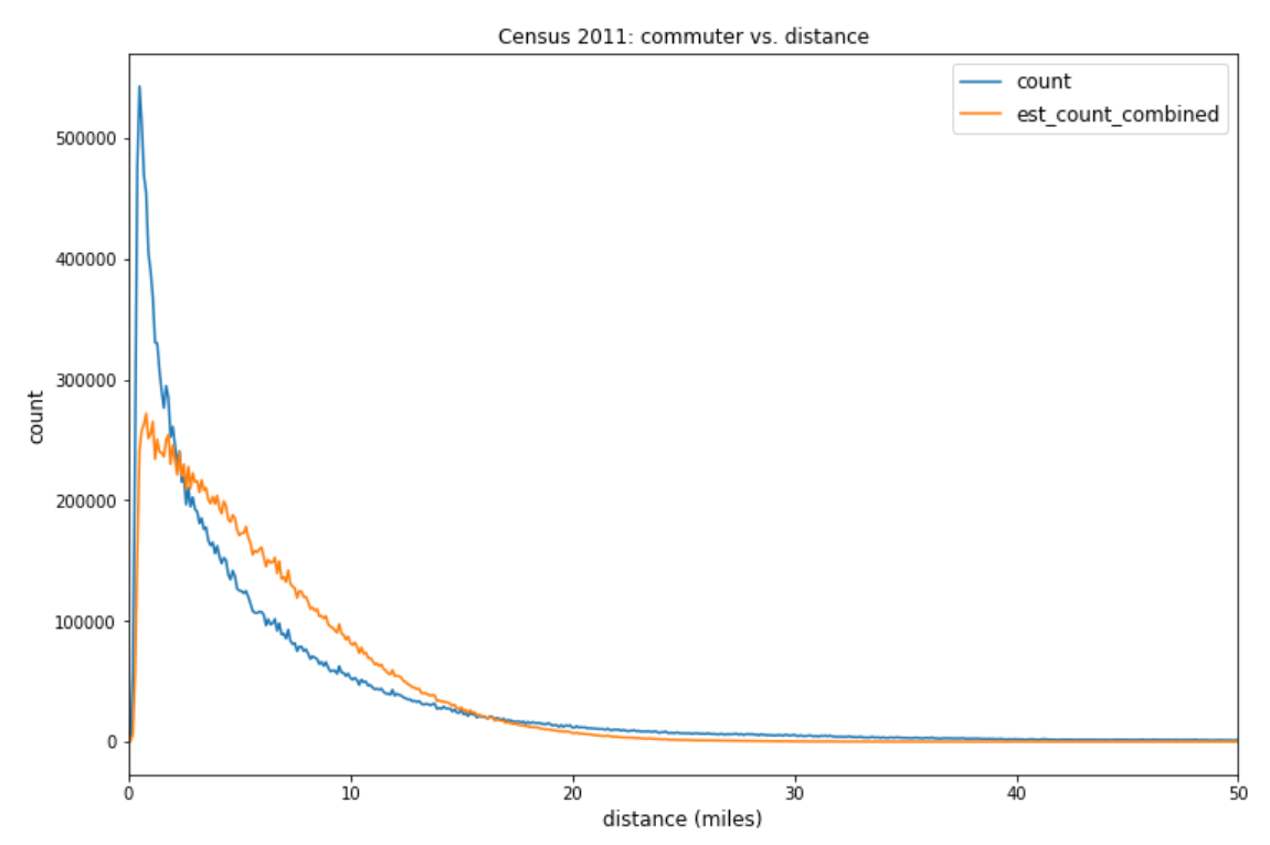
Count: ground truth from 2011 Census travel to work dataset.
Est_count_combined_noseg: estimation from the calibrated cost function.
- These potential improvements have been planned in our roadmap to improve the accuracy of the gravity model for future versions: a more accurate travel distance estimation to reflect the transport network route instead of the current straight-line population weighted centroid distance.
- Another significant improvement will come from segmenting by socioeconomic and demographic characteristics (for example, job type and industrial sectors) and travel modes which will homogenise further the travel distance and account for travel behaviour variations; for instance, research shows that manual workers tend to travel shorter distance when compared with professional and managerial workers.
- One other approach is to apply cost dumping to reflect less sensitivity to cost for longer travel distances; a proxy of cost damping can be segmenting by travel distances (for instance, short, medium, and long-distance travels) and estimate separate parameters for each distance band.
- Introduce alternative measures to travel distance specifically generalised costs, which is the combination of travel time and travel monitory costs accounting for variations in value of time.
Doubly constrained module
In the doubly constrained model, all the estimated \(O_i\) and \(D_j \) must satisfy Equations (6) to (8). That is, the total number of the population aged 16 years and over who are in employment and travel to a fixed workplace should equal to the total number of the employees attracted to a fixed workplace.
\(O_i =∑_{j=0}^{N-1}OD_{ij} \) (6)
\(D_j =∑_{i=0}^{N-1}OD_{ij} \) (7)
\(∑_{i=0}^{N-1}O_i =∑_{j=0}^{N-1}D_j \) (8)
Where N is 7201 MSOAs in England and Wales.
If the total of production does not equal the sum of attraction, the attraction is normally rescaled to ensure that the model is balanced.
The values of the balancing factors, \(A_i\) and \(B_j\) are calculated here.
\(A_i=1/∑_jB_j*D_j*f(c_{ij}) \) (9)
\(B_j=1/∑_iA_i*O_i*f(c_{ij}) \) (10)
The balancing factors \(A_i\) and \(B_j\) are interdependent; this means that the calculation of one set requires the values of the other. An iterative process is used to calculate and : given a set of values for the deterrence functions \(f\left(c_{ij}\right)\), start with all \(B_j\) = 1, solve for \(A_i\) and then use these values to re-estimate \(B_j\); repeat until convergence is achieved.
Summary of modelling assumptions
Here are our key modelling assumptions:
- for our cost function, we use straight-line distance between population weighted centroids of MSOAs and estimate intrazonal travel distance using the distance to the nearest MSOA
- production for future years, between 2011 and 2021 is calculated based on 2011 Census working population with a fixed workplace and growth in workers from NTEM
- production for 2021 is based on working population from Census 2021 and an estimate of the ratio of workers with a fixed place of work; as the Census 2021 travel to work data does not reflect the pre- and post-pandemic commuting patterns, we estimate the ratio travelling to a fixed workplace using the NTS and latent geographic cluster analysis for each MSOA.
- because of changes in definitions of MSOAs between 2011 and 2021, we estimate the Census 2021 working population at MSOA11 geography using the translation methods described in Appendix B
- attraction for future years is calculated based on 2011 Census and growth in jobs from NTEM
4. Results
This first phase of this project produces the estimation of the travel to work matrices annually from 2012 to 2021 at MSOA level for England and Wales. The matrices are estimated for the usual residents aged 16 years and over and in employment with a fixed workplace in England and Wales. It can also extract estimations of resident workers with a fixed workplace, and employees working in each MSOA in England and Wales, annually between 2012 and 2021. The pipeline can also produce the travel to work matrices from 2022 onwards when new data (such as NTS 2022 and 2023) becomes available.
Figure 7: The travel to work matrix for the year of 2021 assuming pre-coronavirus (COVID-19) pandemic travel behaviours, MSOA covering England and Wales
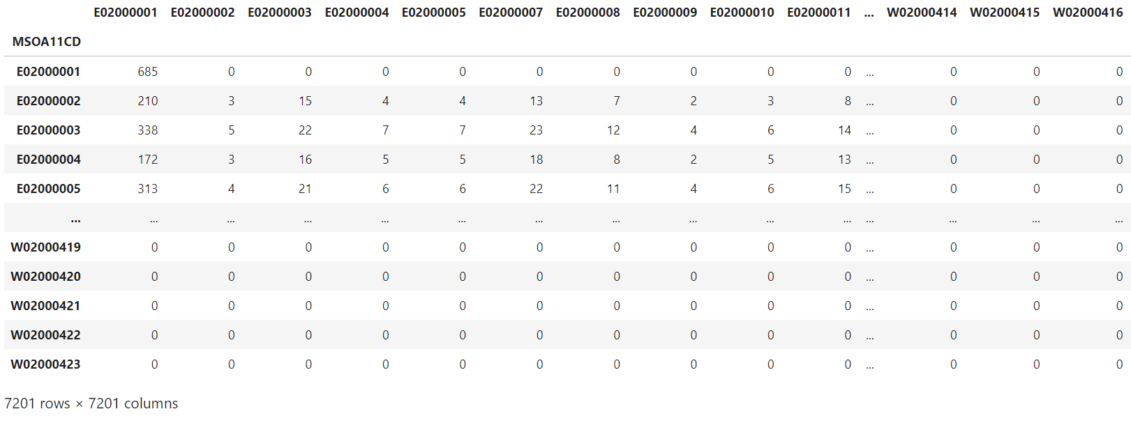
Figure 8: The travel to work matrix for the year of 2021 during the pandemic, MSOA covering England and Wales
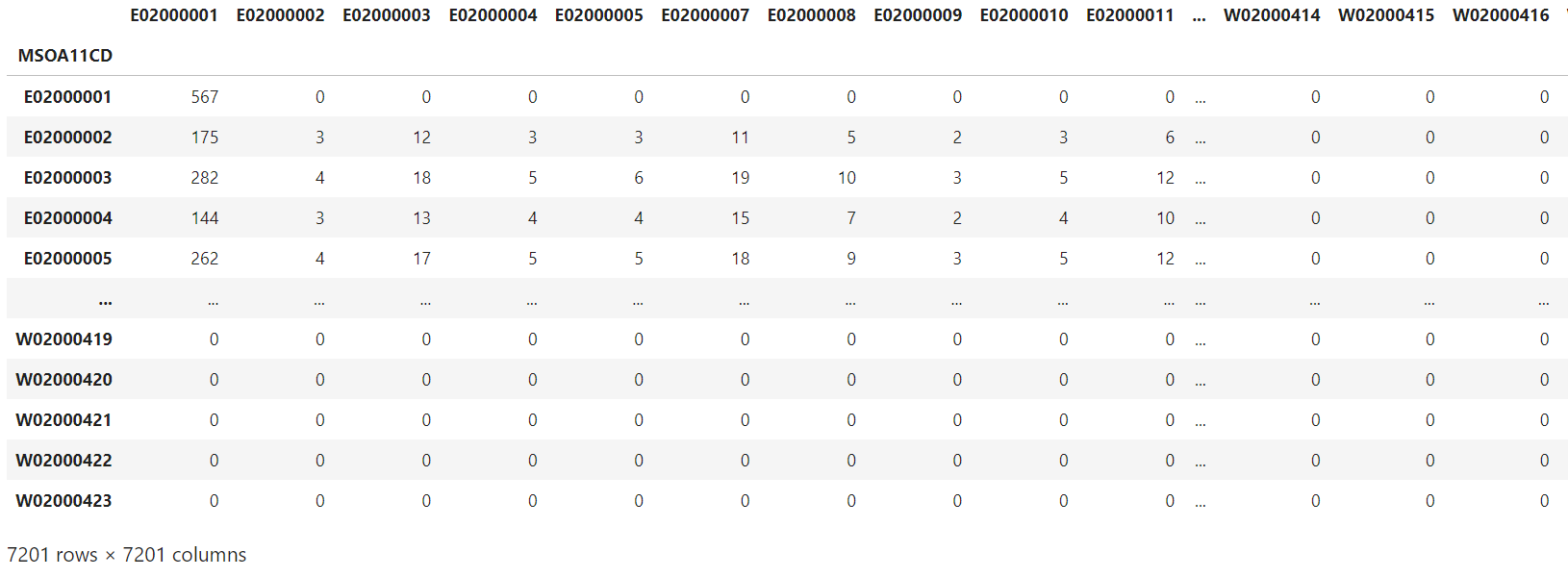
Figures 7 and 8 show the travel to work matrices for 2021 under the assumptions of pre-pandemic and during pandemic commuting travel behaviours, where the first column is origin, and the first row is destination following 2011 Census MSOA geographical definitions. Corresponding values show the number of commuters travelling between origin and destination. To simulate pre-pandemic commuting travel behaviours, the ratio rti is aggregated from NTS data for 2018 and 2019 to reflect the observed commuting patterns before the pandemic. Analysis of commuting travel behaviour grouped by latent geographic clusters (see Appendix C) shows stable or trivial change over time, so the aggregation of 2018 and 2019 NTS data is close to the assumption of normal travel to work patterns without the pandemic in the year of 2021. To simulate commuting travel behaviours during the pandemic, rti is aggregated from NTS data for 2020 and 2021. For more details, refer to Appendix C. Figure 8 shows a significant drop in the number of resident workers travelling to their normal fixed workplaces compared with Figure 7. For example, 210 people travel from their residential area Barking and Dagenham 001 (E02000002) to their main workplace City of London (E02000001) under the assumption of the pre-pandemic commuting behaviours; it drops to 175 under the assumption of mid-pandemic commuting behaviours.
Figure 9 illustrates the estimated travel to work matrices for 2011 (from 2011 Census) and 2021 (under the assumption of the pre-pandemic commuting behaviours) respectively. The maps represent commuting flow between all home and work locations at MSOA level in England and Wales, with lighter lines indicating more commuters travelling to fixed workplaces. The maps provide a sense check on the estimated travel to work matrices for 2021, produced by the model. This is because, over time, we would not expect commuting behaviour to change dramatically, so we would expect a similar picture to emerge from the travel to work matrices estimated for 2021, as we observe in 2011. The maps do, however, show increased intensity of commuter flow in some areas despite an estimated drop in the total numbers of employees travelling to fixed workplace between 2011 and 2021. This is most noticeable in urban and metropolitan areas, presumably because of increases in the numbers of workers and jobs, exceeding any fall in commuting resulting from a reduction in the proportion travelling to a fixed workplace.
Figure 9: Travel to work flow map, MSOA, England and Wales, 2011 Census and Census 2021 assuming pre-pandemic commuting travel behaviours, respectively
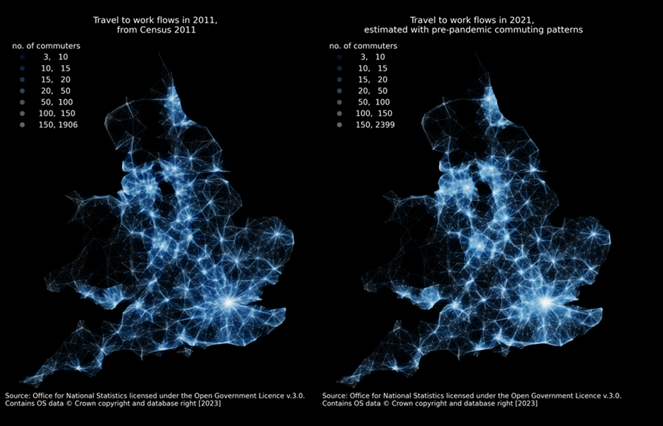
Figure 10. Maps of the number of the working populations who travel to a fixed workplace, MSOA, England and Wales, 2021 under the conditions of pre- and mid-pandemic commuting patterns, respectively
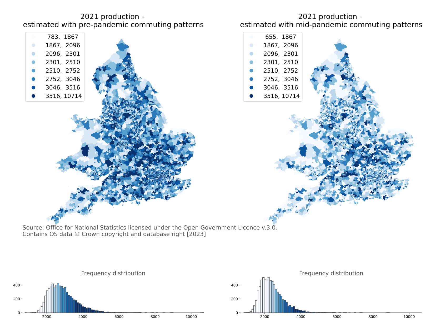
Note: Production is the working population who live in each MSOA and travel to a fixed workplace.
Summing the travel to work matrices in Figures 7 and 8 by rows provides estimations of resident workers with a fixed workplace for each origin MSOA in England and Wales. Figure 10 presents the maps of the number of workers who travel to a fixed workplace at MSOA in England and Wales, 2021 under two conditions: assuming pre- and mid-pandemic commuting patterns, respectively. The pandemic interventions have changed the commuting behaviour where fewer commuters travel to their fixed workplaces than was usual before the pandemic. The degree of changes is likely linked to the type of jobs determining whether employees could work from home.
Figure 11: Maps of the number of employees attracted to MSOA, England and Wales, 2021 under the conditions of pre- and mid-pandemic commuting travel behaviours
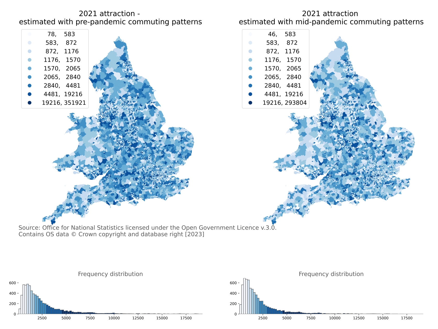
Note: Attraction is the number of employees working at a fixed workplace in each MSOA.
Summing the travel to work matrices in Figures 7 and 8 by columns provides estimations of employees attracted to each destination MSOA in England and Wales. Figure 11 presents the maps of the number of employees attracted to destination MSOA, for England and Wales, in 2021 under the conditions of pre- and mid-pandemic commuting patterns. The pandemic has prevented a significant number of employees from travelling to their usual workplace.
The degree of change in the number of employees with fixed workplaces is likely linked to the industry and type of job of employees. Our roadmap includes extending the model to include segmentation by industry and occupation which will allow us to investigate the changes in more detail. See Section 8 for more details.
Summing the whole travel to work matrix in Figure 8 provides an estimate that 17.6 million people aged 16 years and over who are in employment travel to fixed workplaces under the condition of the mid-pandemic commuting patterns for the year of 2021 in England and Wales. The Census 2021 reports 15.1 million people travelled to a fixed workplace in England and Wales in 2021. The following reasons are likely to cause the difference between the Census 2021 travel to work population (15.1 million) and the estimated result (17.6 million) from the gravity model:
- we estimate the travel to work ratio of workers travelling to a fixed workplace based on NTS data which is collected during a 104-week window between 2020 and 2021, when residents of England and Wales faced varying levels of pandemic-related restrictions
- Census 2021 data were collected for a one-week window on Census Day (21 March 2021) during the lockdown and the furlough policy interventions
- both NTS and census have different guidance on the related travel to work questions
- sample pools and response rates are different – the NTS surveyed a representative sample of 12,852 private households in 2021 and response rates fell during 2020 and 2021 from above 50% pre-pandemic, to 16% in 2020 and 38% in 2021[11]; Census 2021 surveyed all households across England and Wales with a response rate of 97%.
Summing the whole travel to work matrix in Figure 7 provides an estimate that 21.1 million people travel to fixed workplaces in England and Wales under the condition of the pre-pandemic commuting travel behaviours for the year of 2021.
Figure 12: 2011 Census: travel to work options by proportion.
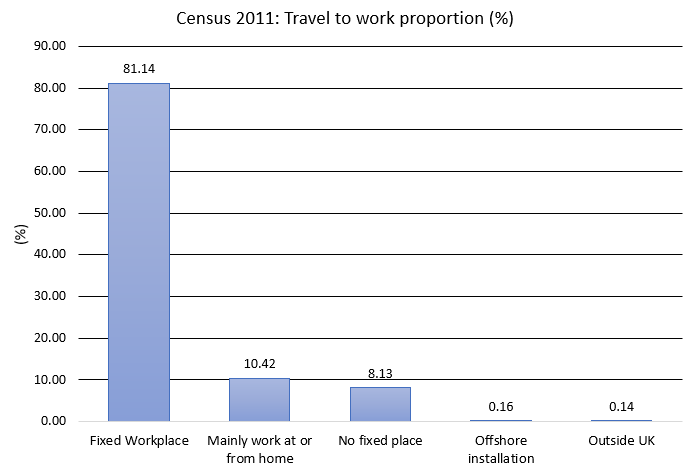
According to the 2011 Census, 26.7 million people were in employment and 21.6 million (81%) people travelled to a fixed workplace in England and Wales. The total population in employment in England and Wales has increased from 26.7 million to 27.8 million from 2011 Census to Census 2021. The Census 2021 reports that 15.1 million (54%) people travelled to a fixed workplace, a significant reduction over 2011.
This is likely because of changes in travel behaviour during the pandemic, particularly related to working from home. Figure 12 shows travel to work options recorded by the 2011 Census by proportion; travelling to a fixed workplace (81%) and mainly work at or from home (11%) are the two main options. The Office for National Statistics (ONS) Annual Population Survey data reports that over the five years before the pandemic, the proportion of people mainly working from home has increased. For the 12-month period from January to December 2019, around 12% of working adults reported working from home at some point in the week before the interview, and around 5% reported working from home all the time, in the UK.
Census travel to work data is used in long-term transport and infrastructure planning, so data as at Census Day would not meet their needs. Although the Census 2021 provided extra guidance to respondents affected by the pandemic on how to respond to travel to work questions. The result indicates that the census travel to work data is a mixture of pandemic and pre-pandemic travel behaviours. The data will also include a substantial number of responses from those who were furloughed, and it is not clear how these furloughed responses were intended.
Our model estimates that 76% working adults (21.1 million out of 27.8 million) travel to a fixed workplace under the assumption of pre-pandemic travel behaviours, which is broadly in line with the trend observed in the years before the pandemic.
It is hard to validate our model outputs, particularly at finer spatial granularity because of data availability and the limited sample coverage at fine spatial granularity of survey-based data, such as NTS. Furthermore, there is little information on post-pandemic travel behaviour. Validation options and limitations are discussed in Section 5.
5. Discussion
This document has described a gravity model to fuse various data to estimate travel to work matrices annually for MSOAs in England and Wales. This is expected to bridge the gaps of temporal granularity of census travel to work matrices and provide an approximation of travel to work matrices for pre-, mid- and post-pandemic travel behaviour where census 2021 travel to work data faces some quality issues because of the influence of the pandemic. This section will discuss issues which affect the quality of results and influence the project.
Validation of results
An unresolved issue for this project is the validation of outputs. Outputs of such models are usually validated by comparison with observed data, such as from surveys. This has not been possible in the absence of a representative survey of travel to work for 2021, such as the context of the Census 2021. We are currently investigating potential datasets which can be used for validation. These include:
- mobile phone data, for example, aggregated footfall data derived from mobile phone users, the usefulness of which is subject to transparent methodology for data generation and representative data for the small area demographic statistics; This data is not yet available to us
- future releases of NTS, which will provide regional data on travel behaviour trends; however, the NTS is not representative at more detailed geographic granularity (for instance, at MSOA level) so cannot be used directly to validate travel to work matrices
- Census 2021 travel to work matrices; the quality is not sufficient for validation but can be used to compare model outputs to identify where substantial differences occur
- a 2019 census rehearsal was undertaken for four areas, Carlisle, Ceredigion, Hackney and Tower Hamlets
- travel surveys have been undertaken by local authorities such as Greater London Authority, Transport for London, and Greater Manchester; these may provide useful validation data
The model will be further improved by segmentation, such as travel distance, travel modes, type of jobs and socioeconomic characteristics. These segmentations will improve the calibration and the quality of travel to work matrices and will result in much higher confidence in the outputs. In addition, segmentation will enable travel to work matrices to be estimated by travel modes and population segments, such as age and occupation. Moreover, incorporating segmentation by socioeconomic and demographic characteristics can help evaluate policy constraints and changes in travel patterns (such as the effect of shifting to work from home or hybrid working by job type and other socioeconomic characteristics post-pandemic). This latter point can contribute into our long-term vision for a cloud-based interactive solution which allows scenario-based analysis.
Data caveats
Data currently used in the model, such as NTS and NTEM, demonstrate low confidence at fine spatial granularity (smaller than LAD, such as MSOA) because of their sample size, response rate and coverage. This will affect the spatial granularity and reliability of the results the model can estimate. We are developing cooperations with DfT to improve the input data quality. We are also planning to add several datasets to this framework including the Labour Force Survey (LFS), Business Register and Employment Survey (BRES) and mobile phone data to improve the model and the quality of the output.
Ground truth for calibration
The model is calibrated based on the ground truth of Census 2011 travel to work data. In a short time period, the calibrated cost function and model can reflect the suitable basis for estimating future year matrices: however, in the long term, the cost function form might shift due to various parameters which are not necessarily accounted for in our model such as significant change in economic, social or technological structure and urban forms. We are investigating how and in which time intervals to recalibrate and rebase the model. One solution is to commission collecting smaller samples (compared to Census) on travel to work or alternatively use of carefully analysed large data sources (or a combination of both) for building the synthetic base year matrices.
6. Conclusion
To bridge the temporal gap of travel to work matrices from census being produced every 10 years and the context of Census 2021 being undertaken during the coronavirus (COVID-19) pandemic, we propose a gravity model-based processing pipeline which estimates the working population and employee growth, calibrates the cost function, and then estimates travel to work matrices for 2012 to 2021, at MSOA level for England and Wales. This model is scalable and flexible to integrate more data and improve the quality of the outputs. We indirectly justify the reasonability of the results using Census 2021 employment data and Office for National Statistics (ONS) employment and labour market data at an aggregated level. Validation at more disaggregated spatial level is currently difficult because of lack of data. We also identified the issues and caveats which affect the model and the results and propose some methods to improve and validate the model in future versions.
7. Future steps
The longer-term vision involves developing a scenario-based modelling approach to generate regular and highly segmented travel to work matrices. The model will augment a wide range of Office for National Statistics (ONS) or available-to-ONS data, such as household, jobs, and travel surveys (including census, IDBR, National Travel Survey, and so on), geospatial data (connectivity, accessibility, rural-urban classification, zonal boundaries, and so on), and large datasets (VOA, Mobile Phone Data, financial transaction data, and so on) and allow scenario-based analysis to enable decision making under uncertainties on future housing market, jobs market, economy, and technology developments. This allows testing “what-if” policy questions and scenario-based analysis for a wider purposes and population segments.
Aligned with the above vision, the possibilities for future work on this project are extensive; these include:
- plan and implement a strategy for model validation (we see this as the highest priority)
- develop better estimation of jobs and population growth using various sets of detailed data and products across the ONS and through developing joined and collaborative plans
- segmenting the model by at least job type (for example, industrial classification, SIC, at workplace end), residential population type (for example, occupation type, SOC, at residential end) and travel distance bands (for example, short, medium, and long-distance trips) to improve model calibration and validation results
- further segmentation by main transport modes including public transport, private modes and non-motorised modes
- incorporate mobile phone mobility data for residential and workplace estimation and travel to work validation
- extend the developed model to include wider travel purposes including leisure and tourism
- build on current spatial model to develop a recursive spatial equilibrium model that can account for major development or restructuring. In the model in our vision, producer and consumer choices adjust to temporal changes in activity churn, background trends, estate development, and transport supply.
- develop a scenario generator which can update model assumptions (for example, proportion of working from home for office-based SICs) under different user-specified scenarios
- developing better spatial visualisation of movements and population
- incorporate other deterrence functions for measuring connectivity in addition (we are currently using travel distance); the first attempt can be developing a generalised cost from combining travel time and distance given the value of time of different socioeconomic and demographic segments
- develop the fully reproducible model on the cloud which can read in the data (for example, mobile phone data), recalibrate the model and produce outcomes given requested scenarios in real time linked to a dashboard for dissemination and report generation
8. Annex
Appendix A: Generating a distance matrix including intra-zonal distance estimations
Summary
This appendix presents the method used to generate an initial cost matrix based on distance between each MSOA pair. The method includes the estimation of intrazonal travel distance using two methods. Method one is estimated from the weighted average travel distance for workers with a fixed place of work using the 2011 Census journey to work data (wf02ew_oa) and population weighted centroids (see Table 1). Method two is a simplified version estimated from the distance to the nearest adjacent MSOA. The second method is required for the estimation of the 2021 origin-destination matrix, as Census 2021 journey to work data is not yet available for the calculation of a weighted average.
Method
The distance matrix provides a distance value in miles or kilometres for each origin-destination pair in the form of a matrix (for instance, origins in column zero, destinations in row zero). The distance is defined as straight line distance between population weighted centroids for each MSOA pair. Intrazonal distances, such as where origin and destination MSOAs are the same, are zero and therefore an ad This is important as in the 2011 Census travel to work matrix for England and Wales, 9.7% of all trips are intrazonal.
Intrazonal distance estimation
Method one (census flow weighted average method) – weighted average distance travelled to work within each MSOA.
This method calculates a weighted average distance travelled to work within each MSOA using commuter flows between lower-level geographic zones contained within each MSOA, for example, output area (OA) to workplace zones (WZ) travel to work matrices from the 2011 Census. More specifically, for each OA to WZ pair contained within each MSOA, population weighted centroids are used to calculate distance and the number of commuters is used to calculate the weight. One example is MSOA intrazonal distance = ∑ (distance between each OA -> WZ within MSOA * number of commuters between each OA -> WZ within MSOA) / number of intrazonal commuters within MSOA.
Method two (nearest adjacent zone method) – proportionate to the distance to nearest MSOA (as used by Transport for the North and recommended approach in TAG M2.1 variable demand modelling).
This method is based on the distance to the nearest MSOA using the existing cost matrix. For each origin MSOA, the minimum distance value to all other MSOAs provides the basis of the intrazonal distance estimate (for example, the minimum value in the array of distance values for each row of the cost matrix). The minimum distance is then divided by two to estimate intrazonal distance. MSOA intrazonal distance = distance from MSOA to nearest neighbour * 0.5.
Appendix B: Matrix translation methods for addressing changes in MSOA geography between 2011 and 2021
Summary
This appendix presents the methods used to translate MSOAs and OD matrices from 2011 to 2021 geography and vice-versa. The method can be applied to any of the output area geographies (MSOA, LSOA, and OA) to translate a full matrix, or either matrix axis, for instance, to convert production values (Oi) or attraction values (Dj) between 2011 and 2021 MSOA definitions.
Problem definition
The definition of 2021 output area geography, which are used to provide statistical outputs for Census 2021, have changed over those of 2011. These changes are necessary to reflect changes in household composition within certain areas that have seen significant change, or to reflect changes in administrative boundaries. There are three levels of Census area definitions: output area (OA), which is the lowest level of census geography; Lower Layer Super Output Area (LSOA); and Middle Layer Super Output Area (MSOA) which is the highest-level output area. This annex describes a method and functions that can be applied to any of these output area levels but focuses on MSOAs. For an overview of Census 2021 geography, refer to the relevant census pages on the Office for National Statistics (ONS) website.
Lookup tables are available from ONS Geography, providing a link between 2011 MSOA and 2021 MSOA codes, along with a change identifier (U=unchanged, M=merged, S=split, X=geography or code changes).
Figure A1 shows an example of an unchanged MSOAs. In these cases, both geography and codes remain unchanged between 2011 and 2021. There are 7,080 unchanged MSOAs.
Figure A1: Unchanged MSOA example
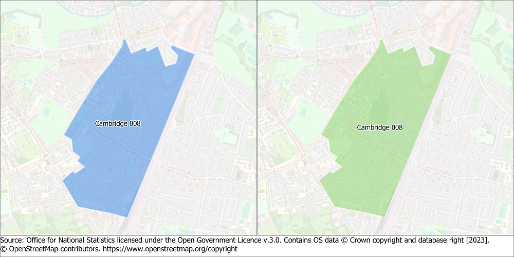
Figure A2 shows an example of merged MSOAs, where one or more 2011 MSOAs become one 2021 MSOA. 40 2011 MSOA become 21 2021 MSOAs.
Figure A2: Merged MSOA example
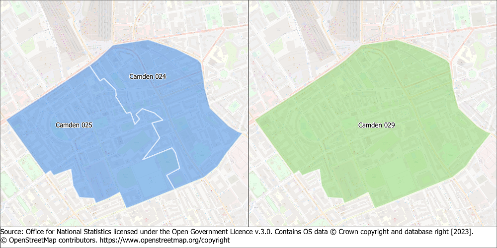
Figure A3 shows an example of split MSOAs, where one 2011 MSOA becomes two or more 2021 MSOAs. 79 2011 MSOAs become 161 2021 MSOAs.
Figure A3: Split MSOA example
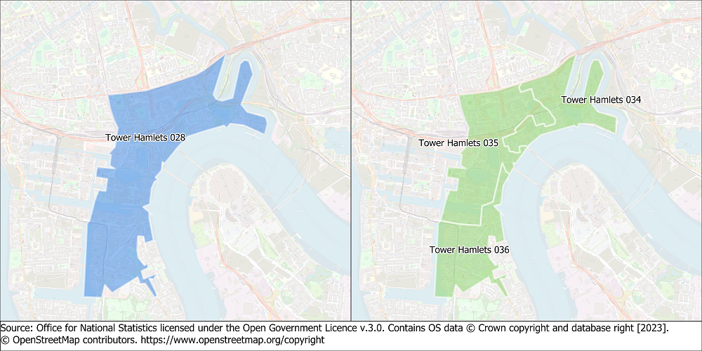
Figure A4 shows an example of changes identified as X, where there are geography or code changes. In this example, a small geography correction has been applied to the 2011 MSOA boundary and code updated. In the lookup table provided by ONS geography, the changes marked as X suggest a one-to-many relationship between 2011 and 2021 MSOAs. This has occurred because of the slight correction to the boundary, triggering a slight change in the boundary of the adjacent MSOA. There are nine MSOAs in this category, although three can be ignored as they represent these adjacent MSOAs that have gained a sliver of geography. This has been confirmed by discussion with Chris Gale (ONS Geography) and by a manual check.
Figure A4: Example of MSOA changes marked as X
Method
The method is described below, with reference to an example OD matrix, shown in Table A1.
Table A1: Example OD matrix
| MSOA11 | E02003726 | E02000189 | E02000190 | E02000891 | E02004947 |
| E02003726 | 35 | 19 | 38 | 42 | 27 |
| E02000189 | 29 | 15 | 36 | 44 | 30 |
| E02000190 | 16 | 42 | 24 | 35 | 30 |
| E02000891 | 43 | 33 | 31 | 49 | 10 |
| E02004947 | 11 | 28 | 41 | 42 | 14 |
The method first generates a lookup table with weights based on the input lookup table of MSOA changes provided by ONS Geography. An example input lookup table is shown in Table A2, referencing the MSOA codes in the example OD matrix shown in Table A1. The lookup table links 2011 MSOA codes with 2021 MSOA codes, with change identifiers.
Table A2: Example lookup table
| MSOA11 | MSOA21 | Change type | Change description |
| E02003726 | E02003726 | U | Unchanged |
| E02000189 | E02007115 | M | Merge |
| E02000190 | M | Merge | |
| E02000891 | E02007114 | S | Split |
| E02007113 | S | Split | |
| E02007112 | S | Split | |
| E02004947 | E02007091 | X | Code change |
Weights are added to the lookup table for those output areas that are split between 2011 and 2021. In this example, weights represent the area of the 2021 MSOA as a proportion of the area of the 2011 MSOA being split. This could be any other value, for example, the number of employees. The weight allows the values from the original OD matrix to be portioned to each 2021 split MSOA. An example lookup table with weights is shown in Table A3.
Table A3: Lookup table with weighting factors
| MSOA11 | MSOA21 | Change type | MSOA11 area | MSOA21 area | Weight |
| E02003726 | E02003726 | U | 20 | 20 | 1 |
| E02000189 | E02007115 | M | 10 | 30 | 1 |
| E02000190 | M | 20 | |||
| E02000891 | E02007114 | S | 70 | 14 | 0.2 |
| E02007113 | S | 21 | 0.3 | ||
| E02007112 | S | 35 | 0.5 | ||
| E02004947 | E02007091 | X | 14 | 14 | 1 |
Table A4 shows an example OD matrix, including the change types and row and column totals.
Table A4: Example OD matrix to be translated, including change types and totals
| U | M | M | S | X | ||||
| MSOA11 | E02003726 | E02000189 | E02000190 | E02000891 | E02004947 | Sum | ||
| U | E02003726 | 35 | 19 | 38 | 42 | 27 | 161 | |
| M | E02000189 | 29 | 15 | 36 | 44 | 30 | 154 | 301 |
| M | E02000190 | 16 | 42 | 24 | 35 | 30 | 147 | |
| S | E02000891 | 43 | 33 | 31 | 49 | 10 | 166 | |
| X | E02004947 | 11 | 28 | 41 | 42 | 14 | 136 | |
| Sum | 134 | 137 | 170 | 212 | 111 | 764 | ||
The first step deals with production, such as the rows of the OD matrix referring to the number of resident workers. This process is shown in Table A5.
Table A5: Translating Oi values
| U | M | M | S | X | ||||
| E02003726 | E02000189 | E02000190 | E02000891 | E02004947 | Sum | |||
| U | E02003726 | 35 | 19 | 38 | 42 | 27 | 161 | |
| M | E02007115 | 45 | 57 | 60 | 79 | 60 | 301 | |
| S | E02007114 | 8.6 | 6.6 | 6.2 | 9.8 | 2 | 33.2 | 166 |
| S | E02007113 | 12.9 | 9.9 | 9.3 | 14.7 | 3 | 49.8 | |
| S | E02007112 | 21.5 | 16.5 | 15.5 | 24.5 | 5 | 83 | |
| X | E02007091 | 11 | 28 | 41 | 42 | 14 | 136 | |
| Sum | 134 | 137 | 170 | 212 | 111 | 764 | ||
| 307 | ||||||||
This process updates the rows in the matrix based on the lookup table and weights described above. The function deals with each change type separately:
- rows in the matrix where the output area code is marked as unchanged are copied to a new matrix retaining values and codes from the original matrix
- the two rows in the input matrix marked as merge are summed to create a single row in the updated matrix
- the one row in the input matrix marked as split is portioned to the three new 2021 MSOAs using the weight
- the one row marked as X are copied to the new matrix and the 2011 code is replaced by the new 2021 code
This results in a new OD matrix with production translated to 2021 MSOAs.
The next step deals with attraction. The same process is applied, but in this case on the columns of the OD matrix, rather than rows. This process is shown in Table A6.
Table A6: Translating Dj values
| U | M | S | S | S | X | ||||
| E02003726 | E02007115 | E02007114 | E02007113 | E02007112 | E02007091 | Sum | |||
| U | E02003726 | 35 | 57 | 8.4 | 12.6 | 21 | 27 | 161 | |
| M | E02007115 | 45 | 117 | 15.8 | 23.7 | 39.5 | 60 | 301 | |
| S | E02007114 | 8.6 | 12.8 | 1.96 | 2.94 | 4.9 | 2 | 33.2 | 166 |
| S | E02007113 | 12.9 | 19.2 | 2.94 | 4.41 | 7.35 | 3 | 49.8 | |
| S | E02007112 | 21.5 | 32 | 4.9 | 7.35 | 12.25 | 5 | 83 | |
| X | E02007091 | 11 | 69 | 8.4 | 12.6 | 21 | 14 | 136 | |
| Sum | 134 | 307 | 42.4 | 63.6 | 106 | 111 | 764 | ||
| 212 | |||||||||
This results in a new OD matrix with both production and attraction translated to 2021 MSOAs.
The method is provided as a Python function with flexibility:
- input variables alpha_id and beta_id dictate the direction of translation; in Figure A10, the alpha_id variable is the 2011 MSOA code and the beta_id is the 2021 MSOA code; reversing the alpha and beta ids allows the translation to work in reverse, for instance, translating a 2021 matrix to 2011 by reversal of merge and split operations
- if a single axis of the OD matrix is provided as the input, for example, totals for Oi or Dj by MSOA, the function translates the single axis to the required geography
Appendix C: Estimating the proportion of workers travelling to a fixed workplace using mobility clusters
Summary
This annex presents the methods used to estimate the proportion of workers travelling to a fixed workplace in 2021, by MSOA. The 2011 Census TTW matrix provides the number of workers travelling to a fixed place of work, which provides our ground truth baseline. We use the Census 2021 to estimate the total number of workers living within each MSOA, but because of the circumstances of the Census 2021 (refer to Section 2 for further details), we cannot rely on this for the estimation of the number of workers with a fixed workplace to calculate production Oi.
Problem definition
The National Travel Survey provides estimates of the numbers of resident workers and the number of resident workers with a fixed place of work for individuals completing the survey. This provides an estimate of the ratio of workers with a fixed place of work, and how this changes over time. While this provides a useful input, the sample size of the NTS means that assumptions cannot be made for small geographies.
Early versions of the model estimated the proportion with a fixed place of work using the average from the NTS for each English region. There are several shortcomings of this assumption. Firstly, it considers workers within each region to have similar working patterns, and while there are noticeable differences between regions, this is an arbitrary assumption based on administrative areas. Secondly, the NTS does not include samples for Wales after 2013.
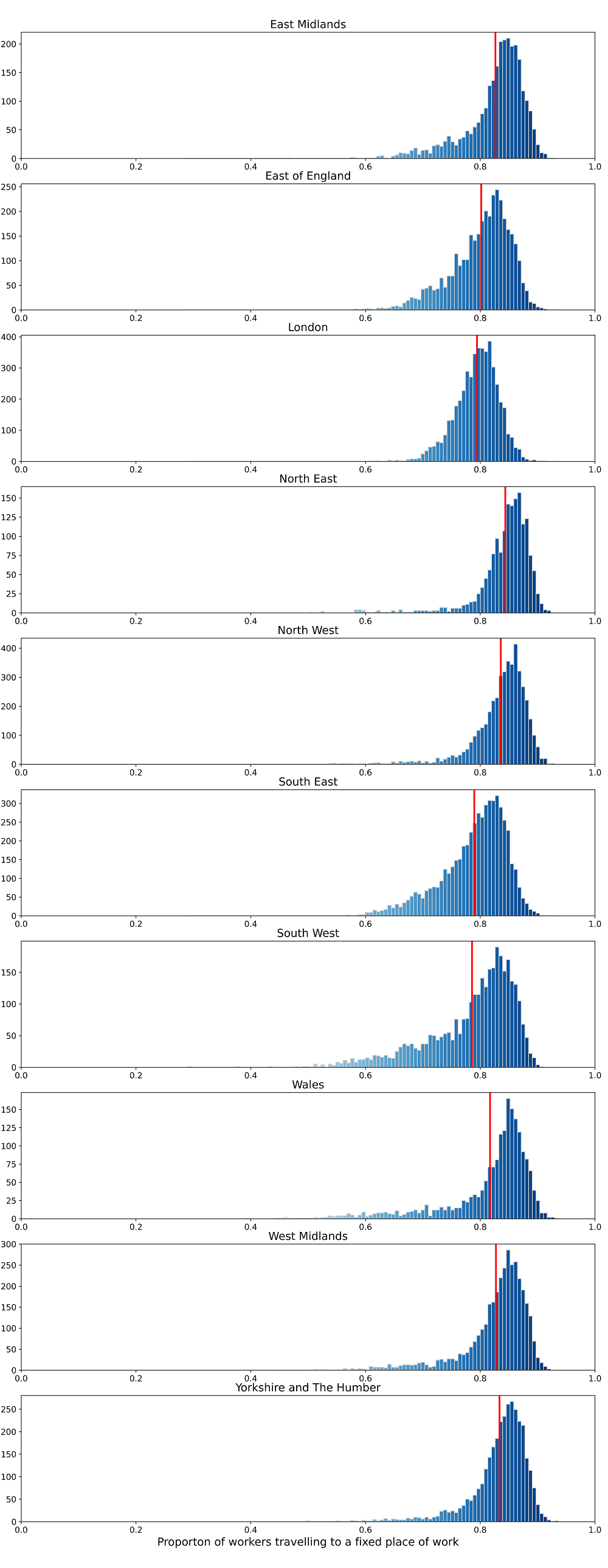
Figure A11 presents the frequency distributions of the proportion of workers with a fixed place of work from the 2011 Census by region. We observe that while there are differences between regions, most have a skewed distribution with large variations in the proportion with a fixed workplace. This highlights the issue with using administrative geographic areas to estimate travel behaviour.
To provide better estimations of the proportion of workers with a fixed workplace, we have investigated the use of latent geographic clusters.
Figure A11: Frequency distributions of the ratio of workers travelling to a fixed place of work (2011 Census) by region
Analysis of latent geographic clusters
We hypothesise that latent geographic clusters, defined by Jahanshahi & Jin [7] and defined in Table A7, provide a better way to estimate the proportion of workers with a fixed place of work compared with regional administrative areas. These latent geographic clusters (mobility clusters) are defined based on a range of land use characteristics including area type, population density and accessibility measures, and have been shown to provide a good estimation of travel behaviour (PDF, 1.87MB).
Table A7: Latent geographic cluster definition
| Latent geographic cluster | description |
| L1. | >70% metropolitan core dwellers |
| L2. | >70% outer metropolitan dwellers |
| L3. | Transition area from L2 to L4 |
| L4. | >70% suburban dwellers |
| L5. | Transition area from L4 to L6 |
| L6. | >70% exurban dwellers |
| L7. | Transition area from L6 to L8 |
| L8. | >70% rural dwellers |
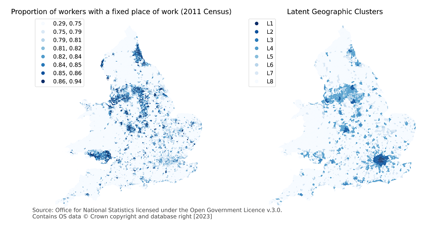
Figure 13 compares the spatial patterns of the proportion of workers with a fixed place of work from the 2011 Census with mobility clusters at LSOA geography. Outside of London the spatial patterns are similar, with more urban areas having a higher proportion of workers with a fixed place of work when compared to more rural areas.
Figure A13. Comparison of spatial patterns of working at a fixed place of work and latent geographic clusters
As London appears to be an outlier, LSOAs within London categorised in cluster L1 or L2 are combined to form a new cluster group. Furthermore, when we observe the frequency distribution of the proportion of workers with a fixed place of work by mobility cluster, two further cluster groups become apparent: urban and suburban areas defined by grouping L2 (excluding London), L3 and L4; ex-urban defined by grouping L5 and L6. The definition of these grouped mobility clusters in shown in Table A8.
Table A8: Grouped mobility clusters
| Latent geographic cluster | description | Definition (grouping of latent geographic clusters) |
| M1. | London | L1 or L2 within London |
| M2. | urban and suburban areas | L2 outside London |
| M3. | ex-urban | L3, L4 or L5 |
| M4. | Rural / ex-urban | L6 or L7 |
| M5. | Rural | L8 |
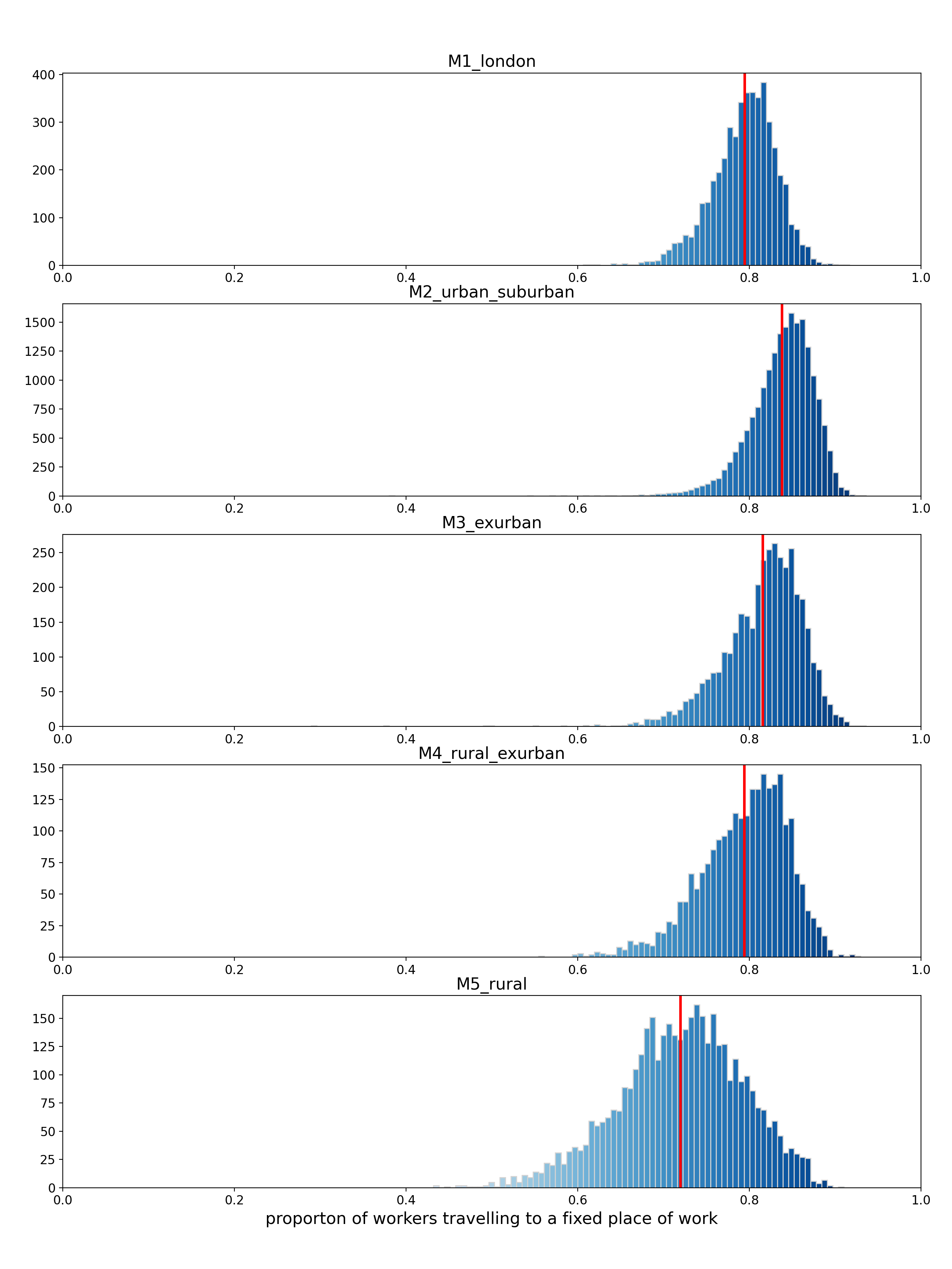
Figure A15 presents the frequency distributions of the proportion of workers with a fixed place of work from the 2011 Census by reduced mobility clusters. We observe that distributions grouped by reduced mobility clusters are more concentrated around the mean and less skewed than when comparing the distributions grouped by regions. This is particularly the case for more urban clusters.
We conclude that, the proportion of workers travelling to a fixed place of work is better estimated using mobility clusters than by administrative regions. This method also provides a way of estimating the proportion for Wales.
Figure A15: Frequency distributions of the ratio of workers travelling to a fixed place of work (2011 Census) by reduced mobility clusters
Method
As our model currently produces travel to work estimates at MSOA geography and reduced mobility clusters are based on LSOA geography, each MSOA is assigned the reduced mobility cluster with the largest population of all usual residents (from 2011 Census). For example, LSOAs within each MSOA are grouped by reduced mobility cluster, and the sum of population is calculated for each group. The reduced mobility cluster with the largest population is assigned to the MSOA. In cases where population is equal amongst reduced mobility (in this case one MSOA contained two clusters with equal population) cluster groups, the highest level, that is, more urban, reduced mobility cluster is assigned to the MSOA.
We use the NTS to estimate the proportion of workers with a fixed place of work. The average proportion at each reduced clusters is shown in Figure A16. The time series shows a significant drop in the proportion of workers with a fixed place of work in 2020 across all mobility clusters. This trend seemed to occur earlier for London, and in urban, suburban, and exurban areas, the trend is mostly stable until 2019. Rural areas show less stability in the proportion, but this can be due to sample size of NTS data in rural area for each survey year.
Figure A16. Time series of proportion of workers with a fixed place of work by mobility cluster from the NTS
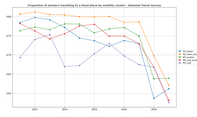
As the primary output of the model is TTW matrices for 2021 excluding coronavirus (COVID-19) pandemic effects, the average proportion of workers with a fixed place of work is estimated by averaging the value for multiple years prior to 2020. This is a parameter that can be adjusted, but we start by taking the average for years 2018 and 2019. To compare pandemic effects, this can be adjusted to 2020 and 2021.
These average values are assigned to each MSOA based on the mobility cluster associated with the MSOA. To estimate the total number of workers with a fixed place of work in 2021, this proportion is multiplied by the Census 2021 total resident employment.