Data science for the public good

1. Introduction

The digitisation of organisational systems has resulted in easier collection and analysis of the information. However, many organisations still store data that was manually collected in paper format, perhaps in scanned images, or entered into a system without quality controls. This is particularly problematic when the data consists of free-text variables. Spelling mistakes, plurality and the use of redundant special characters can prevent large lists of items or products being processed without a complex and extensive pre-processing stage which is often manually intensive. In the case of text data that classifies products, the granularity of classification could also vary considerably.

Natural language processing (NLP) offers a suite of techniques used to make sense of textual information and render it into a structured and well-defined product that can be further analysed. Through algorithmic metrics such as the Jaccard measure and Levenshtein distance, the syntactic closeness of words can be measured to gain an understanding of similarity. Some words are not syntactically similar but share a contextual or semantic relationship and can be evaluated through defined taxonomies (for example WordNet) or by one of the various word embedding methodologies (for example word2vec, GloVe, FastText).

This paper details a processing pipeline for noisy free-text data and produces a well-structured and hierarchical dataset. In the specific application to ferry data, resulting categories of products would ideally be mapped to the international taxonomy used for trade goods, the Harmonised Commodity Description and Coding System (HS2) taxonomy, as used in the UK Trade Tariff tool.

2. Overview of the Optimus processing pipeline

The processing pipeline has several stages that are detailed in turn below. Figure 1 illustrates the steps in the optimus pipeline.

Figure 1: Overview of the Optimus processing pipeline

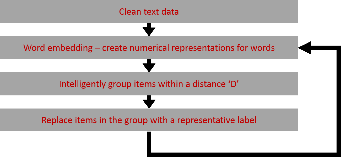
The data first has some basic cleaning applied to it. Special characters and numbers are removed, uppercase characters are replaced with lowercase characters and a custom list of words that are deemed to not hold significant contextual signal are encoded to a sufficiently small string so that when the information is embedded they do not contribute their full weight. Words like products or equipment are common throughout the data and so this encoding strategy reduced their weight in the embedding process.

Following the cleaning process the text descriptions are converted to a numerical form by utilising a word embedding model. The numerical representations are then clustered based on density and finally, a relabelling pipeline attempts to automatically produce a representative group label that replaces the text descriptions of items within a group.

Once group labels have been generated for descriptions that were close together enough to be clustered and relabelled, the process is repeated. With each repetition we widen the net around each point and allow points to cluster with larger diameter.

At the end of each iteration, any items that were successfully mapped to a representative group label for all future iterations are replaced whereas any that did not have a group label generated are persisted.

Each of the stages of the pipeline are now discussed in detail.

Word embeddings

Traditionally, text is analysed by tokenising words and representing them as vectors of a length equal to the number of distinct words in the text where each position in the vector keeps a count of a specific word or ratio of a word to number of documents (term frequency – inverse document frequency). Through this representation, sequences of words can be analysed to understand relationships enabling classification of text, based on word associations. The same word representations can inform generative models that are developed to perform tasks such as sentence generation.

More recently, methods have been developed that represent words as continuous vectors in high-dimensional space but are typically much more efficient than discrete binary vectors. These continuous word embeddings aim to capture contextual information and relate words through specific vector trajectories.

There are several language models that represent text by embedding words in a continuous high-dimensional vector space. The methods used to construct these vectors make them particularly powerful in capturing semantic information between words. Particularly, the continuous bag of words (CBOW) and skip-gram models attempt to maximise the semantic information in the embeddings. Generally, given a collection of sentences, a CBOW model will try to predict a word based on the surrounding words whereas the skip-gram model aims to predict surrounding words for a given word.

FastText extended the skip-gram model to consider character n-grams so that words in the training data were represented as the set of their character n-grams. This subword information skip-gram (SIS) model enables vectors to be developed for any words, not just those that appear in the training data because it can calculate the vectors for the set of character n-grams that make up a word. This also makes the model capable of handling minor syntactic variations such as spelling mistakes and plurality because the list of character n-grams of a word and the corresponding list for a mis-spelling would be similar.

Publicly available pre-trained FastText models have been released in many different languages. The pipeline utilises one of these pre-trained models that has been trained on the English language Wikipedia corpus. The model produces 300-dimensional word embedding vectors by default (this is specified when training a model and is an arbitrary number chosen as a trade-off between training time and amount of contextual information captured by the embedding).

Figure 2 shows a T-SNE two-dimensional visualisation of the embedding space concentrated on an area containing text describing cars and other vehicles. In this space, several important sub-clusters can be identified, for example there seem to be reasonably well defined sub-clusters for Toyota cars, Nissan cars and Citroen cars.

Figure 2: T-SNE plot of embedding space focussed on an area showing transport products

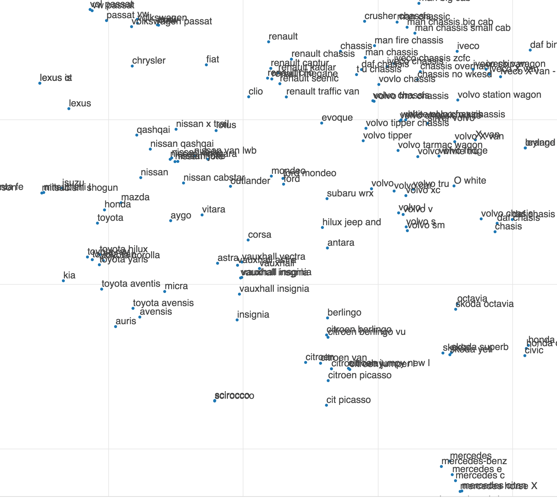
Furthemore, the level of context captured by the model is apparent. For example, it seems cars or brands from Japan are more closely grouped with each other than with other car brands (toward the lower left area shown in Figure 2).

3. Hierarchical clustering

Following the production of vectors for each item description, a hierarchical clustering algorithm is applied to the vectors where Ward’s minimum variance method is used as the objective function.

The product of clustering is visualised as a dendrogram in Figure 3. The closeness of items is indicated by the horizontal distance from left to right to the point where two items’ groups merge.

Figure 3: Dendrogram showing the result of the first iteration clustering for a dataset of product descriptions

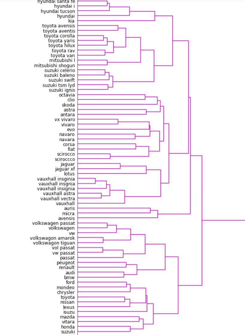
The two closest items that are visible in this dendrogram are “vaxhaull insginia” and “vauxhall insgnia” which are two mis-spellings of “vauxhall insignia”. From the hierarchical structure an attempt is made to produce generalised labels for each subcluster formed within a specified distance. For example, in the example above the two mis-spellings may be replaced with the generalised label vauxhall if some decision threshold is satisfied.

4. Generating cluster labels

As described above, clusters can form either due to their semantic or syntactic similarities. Each cluster is filtered based on a sequence of metrics that determine how a representative label for the cluster should be generated. Each metric aims to identify different patterns in the item descriptions in a cluster in order to handle them in the most appropriate way.

The metrics are considered in a specific order so that small syntactic differences are considered first and with semantic evaluation as the last step. This ensures that small variations such as spelling mistakes and plurality are standardised as a priority before considering clusters that formed based on their contextual content.

Each cluster is sequentially evaluated against the four metrics discussed below until a decision threshold is satisfied. The cluster subsequently has a label automatically generated using an appropriate method detailed below. Figure 4 shows the sequence of evaluators and examples of how labels are generated.

Figure 4: Auto-generating cluster labels with a sequence of evaluators

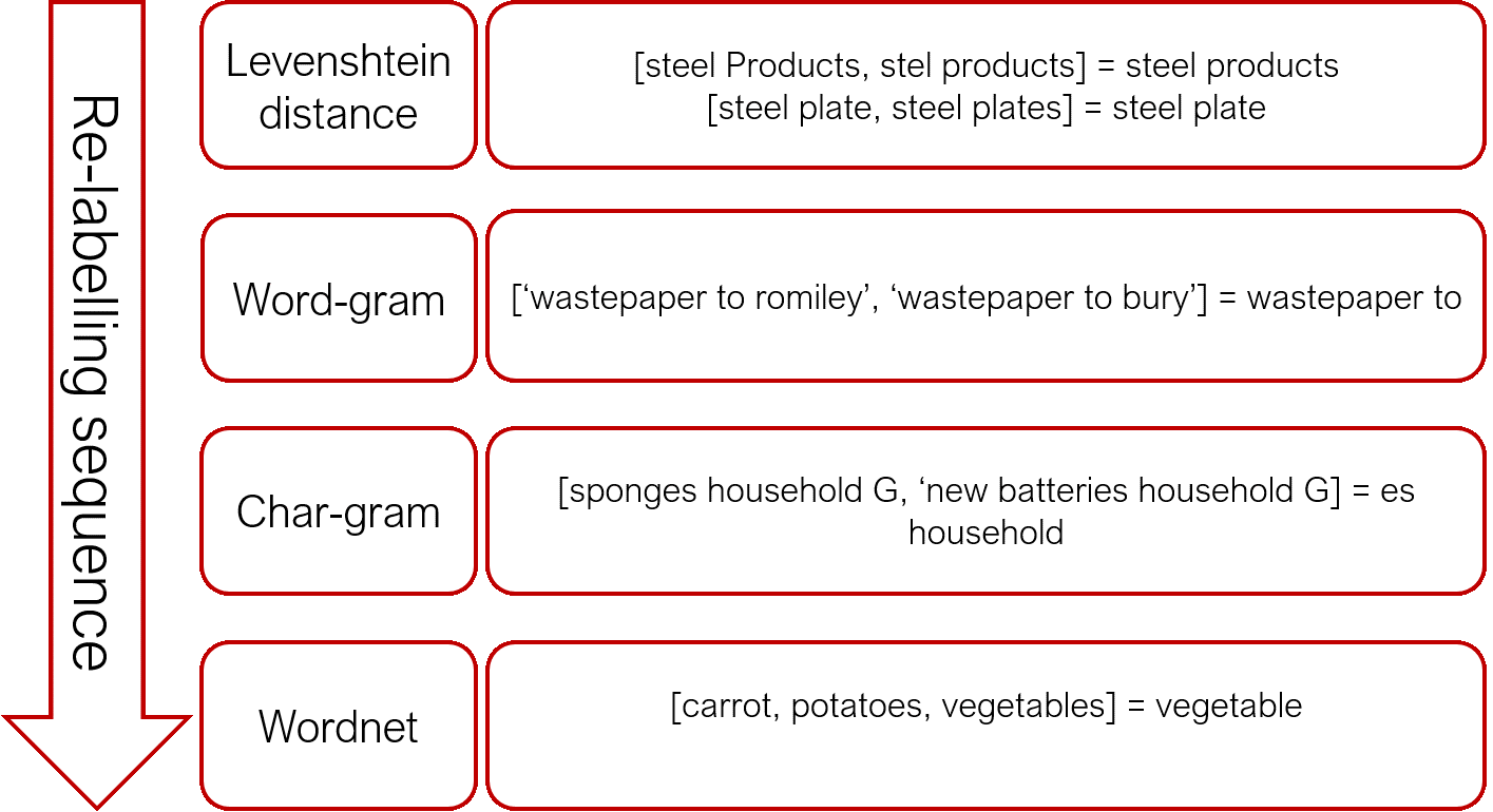
The resulting label for each evaluator is discussed in the section below in detail but summarised as,

1. Levenshtein distance – the most frequent item in the data
2. Word-gram – a sufficiently long and frequent word combination for item descriptions in the cluster
3. Char-gram – a sufficiently long and frequent sub-string for item descriptions in the cluster
4. Wordnet – the lowest common ancestor in a hierarchical tree of word “meanings”.

These evaluators are discussed in detail below.

5. Decision process - the four evaluators

Let us define a Let us define a cluster C that is a set of n strings S so that

 \[ C = \{S_1, S_2,\dots, S_n\}. \] \( \)

1. Average pair-wise Levenshtein distance

The Levenshtein distance is the minimum number of single character operations that need to be made to make two words the same. For example, SAT and CHAT has a Levenshtein distance of two as SAT can become CHAT through two character operations, first a replacement and then an insertion so that (SAT -> CAT -> CHAT). Our calculations use a modification of the standard Levenshtein distance, where transposition of adjacent characters is considered as only one operation rather than two (a removal in one position and an insertion to the opposite side of the adjacent character) – this is traditionally referred to as the Levenshtein-Damerau distance but we will use the term Levenshtein distance here to mean this.

The Levenshtein distance between two strings i and j is denoted L_i,j. For some threshold T_l, the cluster satisfies the average pair-wise Levenshtein distance L_c when

\[ \hat{L}_C = \frac{1}{n}\sum_{i, j \in C} \rho_{i,j} \leq T_l, \qquad \rho_{i,j} = \left\{ \begin{array}{ccc} 0 & if & I_i=I_j \\ L_{i,j} & if & I_i \neq I_j \end{array}\right. \]

2. A suitable word-gram

If syntactic differences are not small enough to satisfy the first condition, then an attempt is made to identify a suitable word-gram from the items in the cluster to label the cluster. Each item I in the cluster C consists of a set of m words (or a sequence of space-separated strings) so that,

\[ \forall I \in C, \quad I = \{w_1, w_2, \dots, w_m\}. \]

For an item I, the bag of all word-grams W, can be denoted as

\[ W = \left( \begin{array}{c} I \\ k \end{array} \right)_ {k=0}^{m} = \{\omega_1, \omega_2, \dots, \omega_p \} \]

that is the bag of all k-combinations of words in an item I. To identify a suitable label to represent the cluster of items, the product of the length of a word-gram w and its frequency across all items I is considered. Finally, the product is normalised by the length of C to ensure that the word-gram is sufficiently representative of the cluster when satisfying some threshold T_w, so that,

\[ \frac{1}{n}\max_{i,j \in C}\left(\sum_{i,j}\delta_{i,j}^2\ln|1+\omega_\alpha|\right) \geq T_w, \]

where

\[ \forall \omega_\alpha \in i, \forall \omega_\beta \in j, \qquad \delta_{i,j} = \left\{ \begin{array}{ccc} 1 & if & \omega_\alpha=\omega_\beta \\ 0 & if & \omega_\alpha \neq \omega_\beta \end{array}\right. \]

If the threshold is satisfied, then the combination of word-grams is used as the group label.

3. A suitable character n-gram label

If there are no word-grams that satisfy the threshold T_w then character sequences are assessed to find a sufficiently long and frequent sequence that can be used as a label for the cluster of items.

For each item I the bag of all ordered character sequences X is denoted as,

\[ X = \{x_1, x_2, \dots, x_q\} \]

The bag of character sequences considered for the cluster label is restricted so that,

\[ X = \{x_1, x_2, \dots, x_q \quad | \quad 3 \leq |x| \leq 20\} \]

The a function of the product of the length of the character sequence and its frequency across all items I in cluster C is considered to identify the best candidate character sequence. The character sequence is then used as the label if the threshold T_x is satisfied so that,

\[ \quad \frac{\hat{L}_{C}}{n} \max_{i,j \in C} \left( \sum_{i,j} \left(\Delta_{i,j}^2 \right) \ln|1+x_\alpha| \right) \geq T_x, \]

where

\[ \forall x_\alpha \in i, \forall x_\beta \in j, \qquad \Delta_{i,j} = \left\{ \begin{array}{ccc} 1 & if & x_\alpha=x_\beta \\ 0 & if & x_\alpha \neq x_\beta \end{array}\right. \]

The average cluster Levenshtein distance is used as a normalisation factor to consider how similar terms are within a cluster. The more dissimilarity across the cluster then the longer and more frequent the character sequence is required to be. If the equation is satisfied then the corresponding labels are used as the group label for items within that cluster.

4. WordNet search

To find the lowest common hypernym to all words in a cluster of item descriptions there needs to exists a common word between the sets of hypernyms. For each string S E C there is a set of r hypernyms H_s where,

\[ H_S = \{h_1, h_2, \dots, h_r\}, \]

and so

\[ \forall S \in C, \quad \exists h_i : h_i \in H_S. \]

Providing this condition is satisfied, let d_i denote the minimum distance of a common hypernym h_i from a string S in the tree of hypernyms. The group label L is then chosen to be

\[ L = \min_{h_i}\sum_{S} d_i \]

that is the minimum cumulative distance between a common hypernym d_i and each string S.

6. Relabelling in practice

The relabelling evaluators attempt to automatically generate appropriate generalised labels for the clusters which works reasonably well but does have limitations.

The main pipeline is iterated, each time having the distance within which items are clustered incremented (this is D in Figure 1). If this distance limit is too high then meaningful and good quality clusters begin to merge and form clusters that are less meaningful. In some cases, the generalised label can become very abstract, or meaningless, whilst the quality of the items in the actual cluster are very sensible.

Another issue in practice is that WordNet does not recognise brand names. The consequence of this is while Carrot, Potato and Parsnip will be replaced with Vegetables, items that consolidate to brand names will not have anything returned from the WordNet query as a suitable label. The consequence of this is that the final dataset will have several well-defined clusters for the same items, for example, the cars in the data set will be contained in multiple clusters with different names such as Nissan, Toyota, Vauxhall and never generalise beyond these labels.

A post processing web-app has been developed to allow a user to apply some post processing to the data set to refine labels and clusters.

7. Post-processing web application

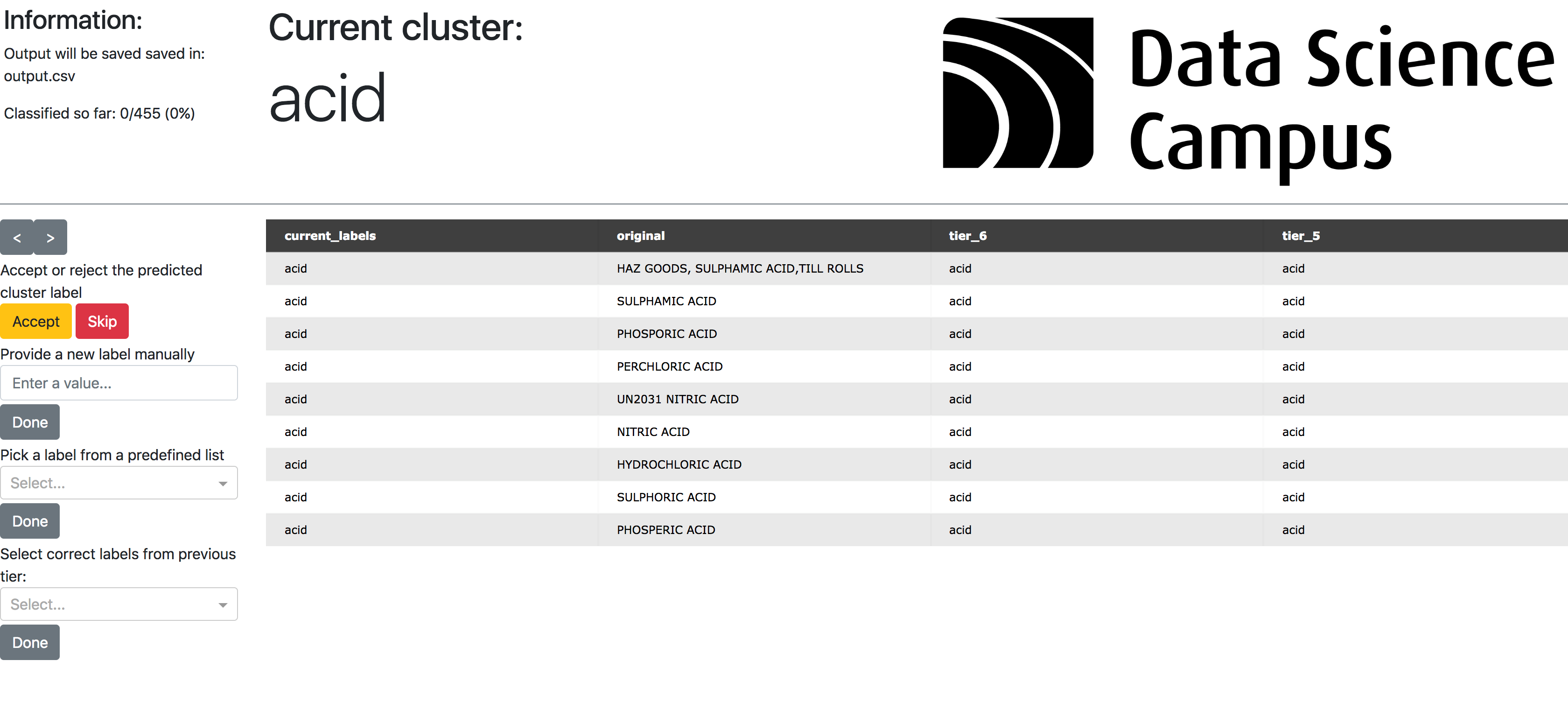
The web app allows a user to cycle through all of the clusters that have formed at the highest tier produced by the optimus pipeline (this is denoted by the current_labels column in Figure 5). The user can view the original item description as well as the other tier classifications produced by the pipeline.

The current cluster and label can either be accepted, rejected as a meaningful cluster or be accepted and have a custom label entered to replace the automatically generated label. This allows consistent labels to be applied across the data set for issues like the same items having different names, for example, clusters for Nissan, Toyota and Vauxhall.

Additionally, lower tiers can be explored and clusters can be broken down into several smaller and more well-defined clusters if the user chooses.

8. Optimus python package

The optimus processing pipeline has is available for use as a Python package on the Data Science Campus optimus Github repository.

9. Conclusion

The optimus pipeline uses modern natural language processing techniques to structure messy short text descriptions that have been collected in an uncontrolled manner. The pipeline performs particularly well on data that consist of short precise items such as shopping lists, essentially noun dominant text.

The fastText model that the pipeline is developed around takes care of much of the structuring by implicitly dealing with impressive amount of noise and variation within the text, although in some cases this does lead to issues. For example, a mis-spelling of wine where the e has been dropped will result in the item win being embedded. This will be embedded in a completely different region of the embedding space, separately to wine and wines due to the word win being word with a context and meaning of its own. Similarly it is difficult to assess all the cases where a word has multiple meanings, such as tanks.

The pipeline clusters the embedded words at different resolutions. This results in a hierarchy of labels. Our experience of using the pipeline on text describing goods confirms the intuition that in the initial stages of embedding and clustering, where the cluster distance is small, the Levenshtein distance evaluator is used to relabel a lot of items because items with small syntactic variances are likely to be embedded closely. Generally the quality of the relabelling appears to be high.

During later iterations where the cluster distance is larger, the word-gram and character-gram evaluators are dominant on relabelling clusters and don’t appear to maintain the same level of quality in the labels being generated for clusters. This is due to the increased variety of text items within a cluster.

Hypernyms appear to be very good at handling instances where items are grouped closely together entirely based on context. In the example in Figure 4 we saw that carrot, potato and vegetable were grouped together and relabelled as vegetables.

The drop in quality of relabelling for some of the evaluators and the perceived difficulty of quality assuring the outputs of the optimus pipeline prompted us to develop the post-processing web application. Using the app, an analyst can both verify the quality of the clusters and relabel them to satisfy themselves, or at least understand the level of noise within them.

The decision to compromise full-automation in favour of a quality check and post-processing step enabled the output data to be accepted by DEFRA and used in practice with confidence in their understanding of the quality of the data. This semi-automated pipeline is much more efficient than the alternative of hand labelling each item in the dataset, rather the data is labelled in meaningful batches. Most importantly, this means the process becomes a realistic exercise to label datasets that have hundreds of thousands of records.

Another benefit that optimus offers is as a tool for the vast creation of training datasets for problems where appropriate labelled data to undertake supervised analysis does not currently exist. Once clusters have been processed by the pipeline, the user essentially has a training dataset. Optimus can speed up this process significantly, acting as a stepping stone to turn a completely unsupervised problem into a supervised one where better assessment metrics can be applied whilst training models.

Although not extensively tested, we believe that optimus could be directly applied to other themes other than trade such as health or education data of similar format and quality.

The code for optimus is available via the Data Science Campus optimus Github.