Automated coding of Standard Industrial and Occupational Classifications (SIC/SOC)

Standard Industrial Classifications (SIC) and Standard Occupational Classifications (SOC) classify the economic activities of businesses and individuals. Their correct assignment is vital in the production of accurate statistics, that inform our understanding of changing trends in industry and occupations of the population in the UK.
SIC and SOC codes and their hierarchy require specialist knowledge, so accurate self-assignment by individuals who take part in surveys is challenging. Respondents to surveys are asked to describe their industry and occupation in response to freeform text questions like “Describe your occupation” or “Business Description”, “Job role”, and others. At present, the Office for National Statistics (ONS) uses a coding tool built to compare the processed free-text answers to a continuously and manually updated “knowledge base” of matching rules from text to codes. This tool classifies records recognised in the knowledge bases through fuzzy matching, and the records that cannot be automatically classified are diverted to manual processing by expert coders.
The Census, and many surveys, including the Labour Force Survey (LFS), Coronavirus (COVID-19) Infection Survey (CIS), the Annual Survey of Hours and Earnings (ASHE), the Destination of Leavers from Higher Education (DLHE), need a versatile tool that can process the data with high match rate, accuracy, and cost-efficiency.
Cost efficiency per-query is becoming increasingly important with larger surveys like CIS and census coming online, and for large administrative datasets. Therefore, reducing the amount of expensive manual coding required is an office priority.
This report summarises our work to meet widespread demand for better automated and higher quality solutions to this problem, by using machine learning (ML) methods to improve the match rate and accuracy of automatic classification of SIC and SOC classifications.
1. Aims and objectives
At the Office for National Statistics (ONS), automatic classification of survey responses to Standard Industrial Classifications (SIC) and Standard Occupational Classifications (SOC) currently uses the matching tool GCODE, developed by Statistics Canada. For Census 2021, the ONS developed an in-house tool. The in-house tool uses rules-based, probabilistic methodology that is similar to GCODE, and relies on matching to comprehensive knowledge bases.
The ONS tool was used to successfully classify Census data to SIC and SOC and is used by the Labour Force Survey (LFS) and the Coronavirus (COVID-19) Infection Survey (CIS). Match rates of approximately 65% for SOC and 55% for SIC are being achieved by the tool, at an accuracy rate of over 90% as reported by the product owners.
Whilst accuracy rates are high, the match rate is much lower, with a significant number of records that cannot be automatically classified requiring manual processing by expert coders.
We investigated whether a knowledge-based approach or a data-centric machine learning (ML) one would be more performant as a global solution. This means that consideration needs to be given to the variety of use-cases it could be built for. Accuracy at all hierarchical levels of coding would be the desired output with the solution’s operational cost efficiency to be taken into consideration. This means that the cost of developing, running and maintaining the tool as well as the cost of manual coding needs to be taken into consideration in evaluating solutions.
Therefore, our objectives for this project are to prototype a solution that:
- Is accurate:
- yields confident and accurate SIC and SOC classifications
- yields accurately classified data that can be stored and relied upon in the future
2. Is portable:
- can run on any platform without requiring specialist hardware
3. Is cost-efficient to:
- build
- test
- maintain
4. Minimises the need for manual coding
5. Provides a way to refer the uncodable or unknown records to manual (human coders)
2. Our approach
We propose a solution using machine learning, which aims to capture the power and potential of quality data. For the purposes of simplicity and ease of explanation, we opted for a basic approach using Logistic Regression (LR) applied to a frequency matrix based on uni-grams, bi-grams and tri-grams commonly known as a Term Frequency – Inverse Document Frequency (TF-IDF) representation. More details can be found in the methodology sections. However, we would be keen to try more advanced AI approaches in the future as mentioned in the conclusions.
3. Data collection
The following datasets are used as benchmarks for our experiments between the two proposed solutions.
Census
The Census dataset consists of half a million Standard Occupational Classifications (SOC). We placed greater emphasis on SOC results in this report.
Labour Force Survey (LFS)
A survey of employment circumstances, yielding 300,000 samples of SOC codes gold-coded to the SOC 2020 standard.
Coronavirus (COVID-19) Infection Survey (CIS)
70,000 SOC gold-coded samples from the first four to five weeks of the survey.
Annual Survey of Hours and Earnings (ASHE)
A small set of 819 SOC gold-coded samples.
Destination of Leavers from Higher Education (DLHE) survey
A small set of 879 SOC gold-coded samples.
4. Results and discussion
We compare the machine learning (ML) and knowledge base coding tool methods on match rate, overall accuracy and matched accuracy when applied to these gold-coded datasets. By match rate we refer to the percentage of samples that each approach can confidently classify. By confidently we mean that the probability for a record being of a certain class exceeds an agreed confidence threshold. Matched accuracy refers to the accuracy within the matched subset. All benchmarks that we display in this section refer to validation sets we kept in reserve during ML training.
Match Rate
The % of entries that have been assigned a viable SOC/SIC code e.g. match rate = ((12-2)/12)*100 = 83.3%
Matched Accuracy
The % of entries assigned the correct code out of those assigned a viable SOC/SIC code e.g. match accuracy = (4/(12-2))*100 = 40.0%
Overall Accuracy
The % of entries assigned a correct code out of all records (in ML’s case, before thresholding) e.g. overall accuracy = (4/12)*100 = 33%
The census and Labour Force Survey (LFS) models
Of the 500,000 gold-coded census records, we split 360,000 for training, 64,000 for testing and 75,000 for validation. The selected text features were “job_title”, “occ_job_desc” (the respondent describing their work activities), “business” (business area of the respondent), and “employer text” (name of employing company). The match rate on the validation set was achieved for a target 95% accuracy rate using a global threshold of 0.6. In Table 1 we see the results for both Standard Industrial Classifications (SIC) and Standard Occupational Classifications (SOC) codes for census. The machine learning (ML) tool performs best for both SIC and SOC codes in our comparison tests (see Table 1).
The LFS data consisted of 300,000 records with SOC codes gold-coded to the SOC 2020 standard. The data was split 217,000 training data, 38,000 test and 45,000 validation. For our predictions we used the columns “OCCT” (occupation title), “OCCD” (occupation description), “INDT” (industry title) and “INDD” (industry description). The match rate was again achieved with a 95% target using a global threshold of 0.6.
The results on the test sets (SOC) were 84% overall accuracy for census and 85% overall accuracy for LFS, which incidentally are the same as the validation set results within rounding error. Similarly SIC codes test and validation results were the same at 81%. This indicates that the training sets available had enough samples to learn a universal pattern and that the resulting models could not be biased to the training datasets.
Table 1 Overall benchmark results between ML and coding tool
|
|
Census | LFS | |||||
| Code | Tool | Match Rate | Overall Accuracy | Match Rate Accuracy | Match Rate | Overall Accuracy | Match Rate Accuracy |
| SOC (2020) | Coding Tool (with dependencies) | 0.62 | 0.53 | 0.86 | 0.59 | 0.50 | 0.84 |
| ML Logistic Regression | 0.73 | 0.84 | 0.95 | 0.70 | 0.85 | 0.96 | |
| SIC (2007) | Coding Tool (with dependencies) | 0.57 | 0.53 | 0.92 | N/A | N/A
|
N/A
|
| ML Logistic Regression | 0.76 | 0.81 | 0.92 | N/A
|
N/A
|
N/A
|
|
Table 2 displays results for the Census SOC codes per class for the 10 most populated classes and the last row in the table is the overall result for all classes for both tools. Again, we see the machine learning tool outperforming the existing coding tool in every testing aspect.
The third and fourth columns (ML, Coding tool) show the percentage of the class that each tool could correctly classify and on the fifth and sixth columns (ML Only, Coding tool only) we can see the percentage of correct classifications made by each tool only (for example, ML only 67.8%, means that 67.8% of samples on the validation set could only be correctly classified from the ML tool and not the coding one). There we see that for the coding tool the exclusive correct classifications were in the range of 0.2% to 3.1%, whereas for the ML tool the corresponding range was 20.5% to 87.9%. We made this benchmark to understand whether a hybrid solution would be suitable.
Table 2 Benchmarks per class for the 10 most populated classes. The last row ( overall) is calculated using all available classes
Recall by Class – Census Occupation
| SOC 2020 | Number in Class | ML | Coding Tool | ML Only | Coding Tool Only | Overlap | Difference | Class Description |
| 7111 | 3487 | 96.5 | 29.3 | 67.8 | 0.6 | 28.7 | 67.2 | Sales and retail assistants |
| 6135 | 1710 | 96.6 | 40.5 | 57.0 | 0.8 | 39.7 | 56.1 | Care workers and home carers |
| 9223 | 1451 | 96.1 | 63.0 | 34.5 | 1.3 | 61.7 | 33.2 | Cleaners and domestics |
| 4159 | 1352 | 86.2 | 20.5 | 67.8 | 2.0 | 18.5 | 65.8 | Other administrative occupations N.E.0 |
| 1150 | 1154 | 86.6 | 44.2 | 44.3 | 1.9 | 42.3 | 42.4 | Managers & directors, retail & wholesale |
| 9263 | 981 | 91.3 | 73.7 | 19.1 | 1.4 | 72.3 | 17.6 | Kitchen and catering assistants |
| 2313 | 958 | 96.0 | 81.0 | 15.3 | 0.3 | 80.7 | 15.0 | [Higher & further Ed. teaching professionals] |
| 9252 | 951 | 93.8 | 83.6 | 11.4 | 1.2 | 82.4 | 10.2 | [Shelf fillers] |
| 2314 | 893 | 96.9 | 87.9 | 9.4 | 0.5 | 87.5 | 9.0 | Secondary education teaching professionals |
| 2237 | 817 | 97.8 | 66.3 | 31.7 | 0.2 | 66.1 | 31.5 | [Nursing and Midwifery Professionals] |
| Overall | 72107 | 83.9 | 54.0 | 33.0 | 3.1 | 50.9 | 29.9 |
The Coding Tool Only range is 0.2 to 2.6 this time and ML only ranges from 14% to 70.5%.
In Table 3 we see similar patterns that we observed on the LFS dataset, where the ML solution clearly outperforms. The Coding Tool Only range is 0.2 to 2.6 this time and ML only ranges from 14% to 70.5% .
Table 3 LFS benchmark results per class for the 10 largest classes. The last row (overall) is calculated using all available classes.
Recall by Class – Labour Force Survey (LFS)
| SOC 2020 | Number in Class | ML | Coding Tool | ML Only | Coding Tool Only | Overlap | Difference | Class Description |
| 7111 | 1885 | 96.2 | 26.9 | 70.0 | 0.7 | 26.2 | 69.3 | Sales and retail assistants |
| 6135 | 1412 | 98.0 | 44.6 | 53.8 | 0.5 | 44.1 | 53.3 | Care workers and home carers |
| 9223 | 1052 | 98.1 | 60.7 | 38.0 | 0.7 | 60.1 | 37.4 | Cleaners and domestics |
| 4159 | 892 | 90.0 | 20.9 | 70.5 | 1.4 | 19.5 | 69.2 | Other administrative occupations N.E.0 |
| 2313 | 666 | 95.5 | 44.0 | 52.1 | 0.6 | 43.4 | 51.5 | [Higher & further Ed. teaching professionals] |
| 9263 | 638 | 91.9 | 69.6 | 23.4 | 1.1 | 68.5 | 22.3 | Kitchen and catering assistants |
| 2237 | 604 | 98.3 | 53.2 | 45.7 | 0.5 | 52.7 | 45.2 | [Nursing and Midwifery Professionals] |
| 2314 | 594 | 95.0 | 59.9 | 35.2 | 0.2 | 59.8 | 35 | Secondary education teaching professionals |
| 1150 | 547 | 91.4 | 50.1 | 43.0 | 1.7 | 48.5 | 41.3 | Managers & directors, retail & wholesale |
| 9252 | 527 | 92.0 | 80.3 | 14.0 | 2.3 | 78.0 | 11.8 | [Shelf fillers] |
| Overall | 44430 | 84.7 | 49.6 | 37.7 | 2.6 | 47.0 | 35.1 |
The hybrid models
The hybrid models were trained with a mixture of LFS and census data. These models performed .
The hybrid models were trained with 0.5M census training data and 0.3M LFS data split into 0.68M train and 0.12M test data, an 85:15 split. Once trained, each model was used to classify the validation sets for CIS, ASHE, DLHE, which consisted of 64,000, 819 and 879 gold-coded samples respectively. The following table demonstrates the training data and validation data text fields for each of the models created:
Table 4 Training and validation text features for the hybrid models for CIS, ASHE, DLHE
| DLHE | ASHE | CIS | |
| Training | [‘Job_title’, ‘business’] | [‘Job_title’] | [‘Job_title’, ‘occ_job_desc’] |
| Validation | [‘job_title’, ‘business’] | [‘Job_title’] | [‘job_title’, ‘main_job_responsibilities’] |
The benchmark results are appended in the following table. The resulting human in the loop split was achieved using a variable threshold with a target accuracy of 0.975 on the train-test dataset.
Table 5 Benchmark results for DLHE, ASHE, and CIS for the coding tool and the hybrid Logistic Regression models. The numbers in bold are the highest scores for each category. The blue highlighted numbers are scores without using a match rate threshold, ie. 100% match rate.
|
|
DLHE | ASHE | CIS | ||||||
| Match Rate | Overall Accuracy | Matched Accuracy | Match Rate | Overall Accuracy | Matched Accuracy | Match Rate | Overall Accuracy | Matched Accuracy | |
| Coding Tool | 0.45 | 0.35 | 0.77 | 0.56 | 0.44 | 0.867 | 0.47 | 0.46 | 0.98 |
| Logistic Regression | 0.48 | 0.61 | 0.81 | 0.67 | 0.69 | 0.866 | 0.66 | 0.76 | 0.90 |
In Table 5 we see that for DLHE the Logistic Regression model outperformed the coding tool in all aspects. For ASHE, we see that the matched accuracy is similar, however, the match rate for the LR model is 11% higher and the overall accuracy 25% higher for LR.
Finally, for the Coronavirus (COVID-19) Infection Survey, LR outperforms the coding tool on match rate by 19% and the coding tool demonstrated a 98% matched accuracy compared with 90% for LR. However, again the overall accuracy was higher for the LR model by 30%, and the CIS implementation of the coding tool is unusual, having disabled nearly all fuzzy-matching functionality. Disabling this functionality meant that the tool would only classify direct matches, which in turn results in much higher accuracy than usual, at the cost of match rate, which dropped at 47% compared with 66% for the LR model. The performance for both solutions was lowest on DLHE.
Table 6 A – Recall by Class – Covid Infection Survey (CIS)
| SOC 2020 | Number in Class | ML | Coding Tool | ML Only | Coding Tool Only | Overlap | Difference | Class Description |
| 7111 | 1762 | 89.3 | 58.1 | 33.7 | 2.4 | 55.7 | 31.3 | Sales and retail assistants |
| 4159 | 1737 | 76.3 | 13.5 | 63.4 | 0.5 | 13.0 | 62.9 | Other administrative occupations n.e.c. |
| 6145 | 1610 | 87.6 | 41.8 | 46.8 | 1.0 | 40.8 | 45.8 | Care workers and home carers |
| 2231 | 1502 | 96.7 | 81.8 | 15.3 | 0.4 | 81.4 | 14.9 | Nurses |
| 1259 | 1293 | 42.5 | 8.3 | 34.7 | 0.4 | 7.9 | 34.3 | Managers and proprietors in other services |
| 3545 | 1121 | 82.6 | 37.6 | 45.9 | 0.9 | 36.7 | 45.1 | Sales acc’s & business dev’t managers |
| 4122 | 1117 | 52.2 | 70.1 | 16.3 | 34.2 | 35.9 | -17.9 | Book-keepers, payroll managers. |
| 2424 | 957 | 79.7 | 10.9 | 70.4 | 1.6 | 9.3 | 68.9 | Business & financial project management |
| 2136 | 815 | 84.4 | 61.5 | 24.4 | 1.5 | 60.0 | 22.9 | Programmers and software development |
| 6125 | 721 | 93.2 | 87.7 | 7.1 | 1.5 | 86.1 | 5.6 | Teaching assistants |
| Overall | 64578 | 75.9 | 45.7 | 32.9 | 2.7 | 43.0 | 30.2 |
Table 6 B – Recall by Class – Annual Survey of Hours and Earnings (ASHE)
| SOC 2020 | Number in Class | ML | Coding Tool | ML Only | Coding Tool Only | Overlap | Difference | Class Description |
| 4159 | 41 | 63.4 | 22.0 | 43.9 | 2.4 | 19.5 | 41.5 | Other administrative occupations n.e.c |
| 6135 | 27 | 74.1 | 40.7 | 33.3 | 0.0 | 40.7 | 333 | Care workers and home carer! |
| 7219 | 19 | 68.4 | 47.4 | 21.1 | 0.0 | 47.4 | 21.1 | Customer service occupations n.e.c |
| 4122 | 17 | 52.9 | 64.7 | 5.9 | 17.7 | 47.1 | -11.8 | [Book-keepers, payroll mngrs & wage clerks |
| 6131 | 17 | 58.8 | 35.3 | 23.5 | 0.0 | 35.3 | 23.5 | Veterinary nurses |
| 2237 | 16 | 93.8 | 68.8 | 25.0 | 0.0 | 68.8 | 25.0 | [Nursing and Midwifery Professionals] |
| 7111 | 15 | 66.7 | 20.0 | 46.7 | 0.0 | 20.0 | 46.7 | Sales and retail assistants |
| 3556 | 12 | 91.7 | 33.3 | 58.3 | 0.0 | 33.3 | 58.3 | Conservation & environmental pro’s |
| 5223 | 12 | 66.7 | 16.7 | 58.3 | 8.3 | 8.3 | 50.0 | Metal working prod & maintenance fitters |
| 1121 | 11 | 54.6 | 9.1 | 45.5 | 0.0 | 9.1 | 45.5 | Production mngrs & directors, manufacturing |
| Overall | 819 | 68.9 | 44.0 | 27.5 | 2.6 | 41.4 | 24.9 |
Table 6 C – Recall by Class – Destination of Leavers from Higher Education (DLHE)
| SOC 2020 | Number in Class | ML | Coding Tool | ML Only | Coding Tool Only | Overlap | Difference | Class Description |
| 3554 | 37 | 710 | 46.0 | 27.0 | 0.0 | 46.0 | 27.0 | Marketing associate professional |
| 2319 | 31 | 71.0 | 25.8 | 48.4 | 3.2 | 22.6 | 45.2 | Teaching & other educational professional |
| 2422 | 24 | 79.2 | 50.0 | 29.2 | 0.0 | 50.0 | 29.2 | Finance & investment analysts & adviser |
| 3416 | 24 | 54.2 | 20.8 | 33.3 | 0.0 | 20.8 | 33.3 | Arts officers, producers and director |
| 2434 | 19 | 63.2 | 10.5 | 52.6 | 0.0 | 10.5 | 52.6 | Chartered surveyor |
| 2313 | 19 | 73.7 | 21.1 | 57.9 | 5.3 | 15.8 | 52.6 | Secondary education teaching professional |
| 3413 | 19 | 73.7 | 31.6 | 42.1 | 0.0 | 31.6 | 42.1 | Actors, entertainers and presenter |
| 2431 | 16 | 68.8 | 25.0 | 50.0 | 6.3 | 18.8 | 43.8 | Architect |
| 4159 | 15 | 66.7 | 26.7 | 40.0 | 0.0 | 26.7 | 40.0 | Other administrative occupation |
| 2311 | 15 | 66.7 | 46.7 | 20.0 | 0 | 46.7 | 20 | Higher education teaching professional |
| Overall | 879 | 60.5 | 34.6 | 29.6 | 3.6 | 30.9 | 25.9 |
Table 6 A,B and C shows benchmark results for the 10 largest classes for CIS, ASHE and DLHE. The last row (overall) is calculated using all available classes. The two highlighted rows are the only ones where the coding tool outperformed the ML one.
In Table 6 A,B and C, LR outperforms the coding tool in all of the most populated classes that we benchmarked, apart from one – class 4122 (book-keepers and payroll managers) where the coding tool clearly outperforms LR by a large factor, 17.9% for CIS and 11.8% for ASHE.
Figure 3 gives a graphic overview of the two tools’ performance across different classes, for different datasets. The orange curve represents the number of samples in a specific class in log scale. The classes are sorted by size from the smallest to the largest. The cyan (light blue) curve represents the number of records within a class that the LR matches correctly and the blue one (dark blue) the same for the coding tool.
We observe that the cyan curve for the LR model stays relatively close to the orange curve, however, this is not the case for the blue curve (coding tool), which tends to stay far apart with occasional big drops. The larger the drop, the larger the inability for the tool to predict the associated class.
Figure 3: Per class comparison overview for all classes and for all datasets. The vertical axis is the number of correct classifications for the two tools in comparison. The all curve represents the number of rows per class. The horizontal axis represents the different classes, from the least populated (left) to the most (right)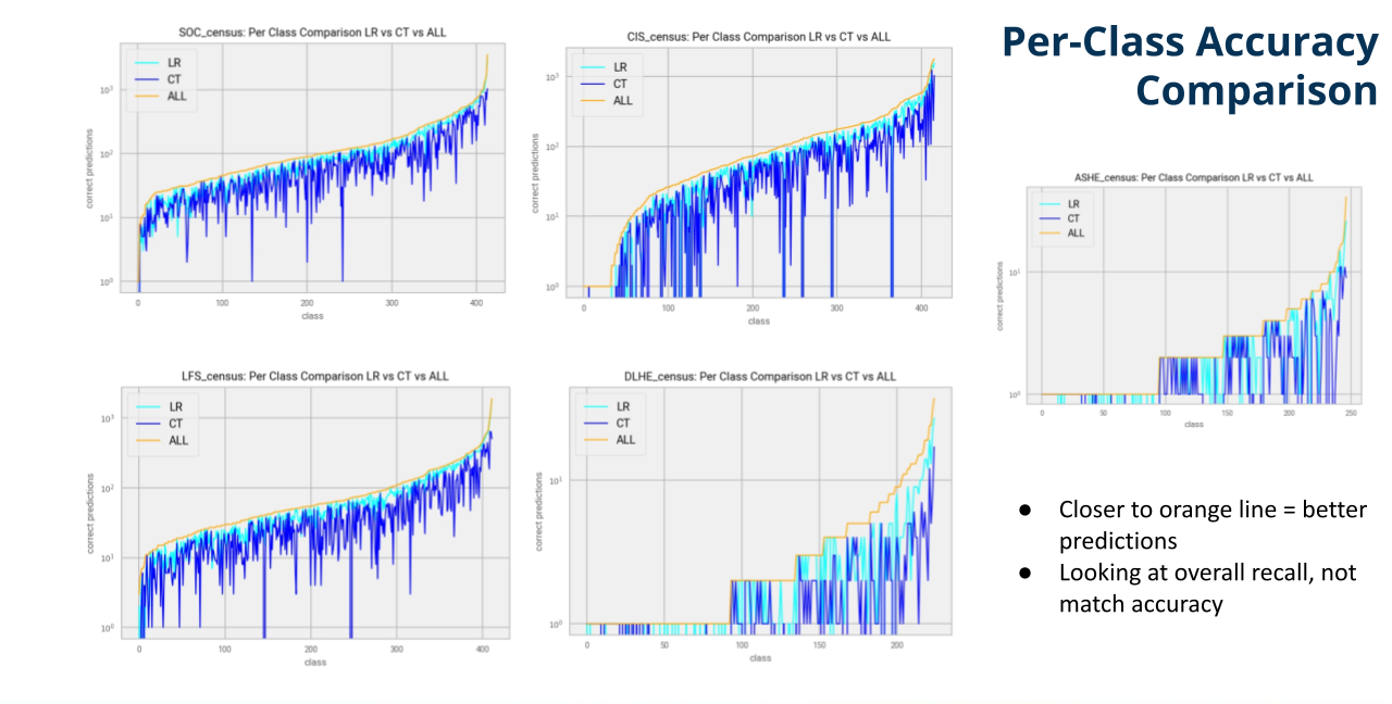
Confidence plots
Figure 4 shows a graphic representation of the confidence of predictions for the LR model in log scale. The horizontal axis is the prediction probability and the vertical represents density, that is, how many right or wrong predictions were made with the associated probability range/bin. The blue bars represent correct classifications and the red bars represent erroneous ones.
The observation we can make on these graphs and especially for the three larger datasets is that there is a clear pattern where the higher the probability the higher the likelihood for a correct prediction, and the other way around. This means that we could make decisions in regard to probability thresholds that could lead to higher accuracy expectations. The pattern is not so strong for our smaller datasets, however, we could argue that this could be because of the size of the datasets being fewer than 900 samples, but we see a similar trend for probabilities over 0.8 and lower than 0.3.
Figure 4 Confidence density plots for the LR tool in Log-scale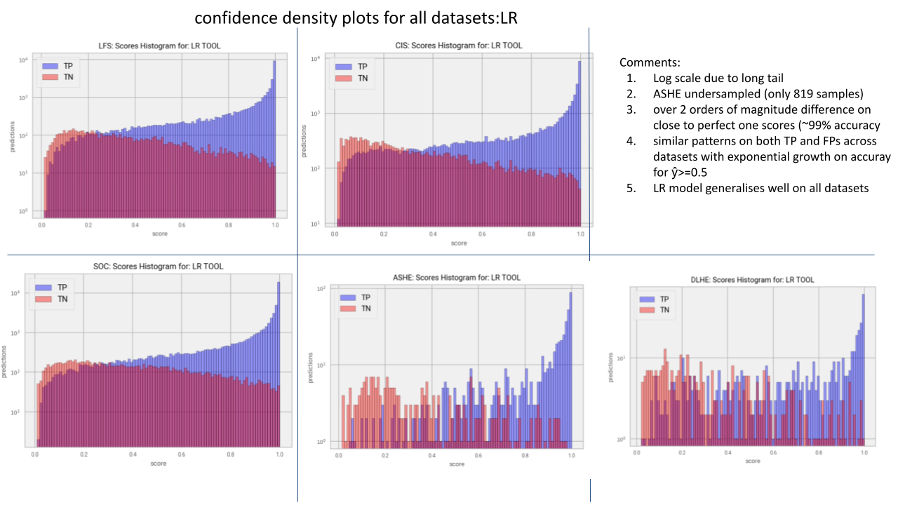
Human in the loop
The option to mix human expert classification and automation is desirable for this project, hence we demonstrate how that can be achieved with a machine learning (ML) system. Initially we opt for a global probability threshold, before expanding to class-by-class solutions.
Global threshold
Figure 5 demonstrates the relationship between match rate, matched accuracy, and general accuracy for each of our datasets for the Logistic Regression (LR) tool.
The green curve overall accuracy is the number of correct classifications divided by all samples, whereas matched accuracy is the number of correct classifications divided by the number of matched samples. In this figure we see a similar pattern, with better results for census, Labour Force Survey (LFS) and Coronavirus (COVID-19) Infection Survey (CIS) and a bit worse for the Annual Survey of Hours and Earnings (ASHE) Looking at this graph, it seems that we could pick a desired probability threshold that could steer our results on future unknown sets towards the target accuracy values. We used these plots to choose a probability threshold of 0.6 for census and LFS models.
Figure 5 A graphical representation of match rate, accuracy and matched accuracy for the LR model and all datasets.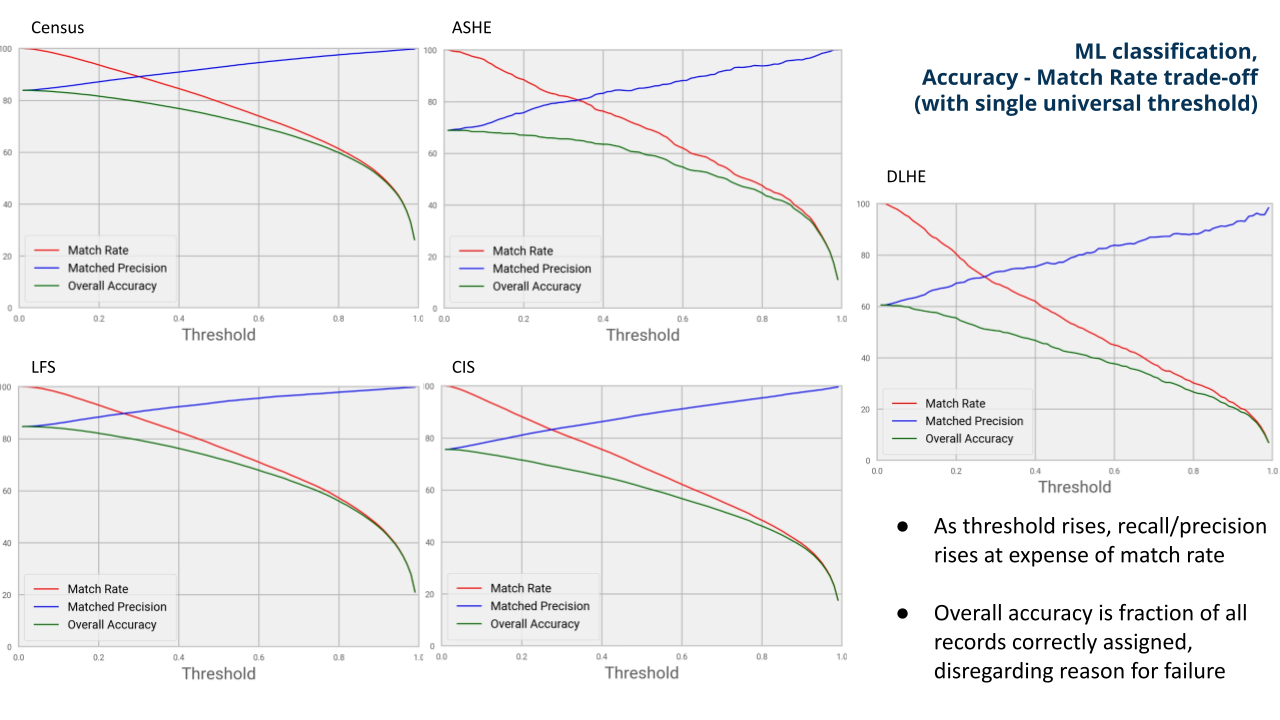
Variable threshold
As an expansion to this idea, we implemented a method of generating probability thresholds by class that aim for a particular accuracy target. Potentially, the model could be more confident in its classifications of some classes than of others and this could be reflected in a per-class threshold map. The aim of this variable threshold is to provide match rates and matched accuracies such that the matched accuracy would correspond to a higher match rate than the one we could get from a global threshold.
Our experiments show that this technique works well for our transfer learning examples (CIS, ASHE, DLHE models) but not so well for census and LFS, where the results were very similar to – and rarely better than – the ones obtained with global thresholds. Another issue we had with this technique was that, although we would calibrate it aiming for 95% matched accuracy, our results never quite matched it, but we got 90% for CIS, 86% for ASHE and 81% for DLHE as we saw in Table 5. The fact that it is a transfer learning exercise could well explain the loss of accuracy.
5. Methods
\( \)The machine learning (ML) classification tool consists of a nested pipeline made of three major pipelines: text processing, feature engineering and model generation. The code for the general tool was partially adapted from ACE2, a general-purpose text classification pipeline developed by the Data Science Campus specifically for this class of problems.
Text processing pipeline.
Text processing consists of the following tasks:
- punctuation removal
- lowercase
- spell check
- split joined up words
- stopword removal
- stemming
Regarding stemming, we chose this over lemmatization as it seems more robust and faster because it is calculated rather than being looked up in lemmatization dictionaries.
Feature engineering
This step consists of embedding the text into a feature matrix prior to model training. We use a TF-IDF (Term Frequency – Inverse Document Frequency) representation of text. We find that having a dedicated TF-IDF matrix per text-field gives us better results than simply merging all text fields and creating a single matrix. Separate matrices allow for different semantics and frequencies between text fields. The TF-IDF matrices were generated for unigrams, bigrams and trigrams for lowest frequency of five documents, then concatenated into a single feature matrix.
Model generation (Logistic Regression with TF-IDF)
Logistic Regression (LR) was chosen for its simplicity, explain-ability, and efficiency when it comes to text classification. The Logistic Regression model, is as simple as learning a weights vector θi and bias b, to satisfy the equation:
\( \)$$ {\hat{y}}_i = (\theta_i) \ X + b $$
Where yi is the prediction probability for each class i, and X is the features (tf-idf) matrix. The weights vector is learned through established and known first or second order optimization methods, in our case LBFGS (Limited Memory for the Broyden–Fletcher–Goldfarb–Shanno algorithm). The objective function for the optimisation was chosen to be the log-likelihood, which is the standard for the Logistic Regression algorithm.
6. Calibrating the match rate
After the model is trained, it is evaluated on an unseen test set in order to assess the model’s ability to generalise. This is when we also estimate the per-class probability thresholds. This is achieved by creating a tuple of probabilities and prediction outcomes (that is, correct, false). Then we pick the maximum sequence whose correct classifications account for a ratio equal or higher to our target accuracy. The resulting threshold map is saved together with the model.
7. Conclusions
As an alternative tool for Standard Industrial Classifications (SIC) and Standard Occupational Classifications (SOC), a machine learning (ML) approach performs extremely well and is naturally suited to this classification problem. Delegation of low-confidence records to manual coders is easily achieved, and the significant accuracy gains ML makes over expert systems using lookup lists should translate to monetary savings against the requirement for manual coders.
A concern for statisticians in some outputs is extremely high accuracy in confirmed matches, given the reliance of multiple statistical products upon the results of the coding system. Figure 5 suggests that in these situations, for sources with suitably large training sets (census and Labour Force Survey (LFS)), near-100% accuracy with a match rate of approximately 50% can be achieved with a high global probability threshold of 0.9. This would still reduce required manual coding, with great confidence in the machine-coded portion of the output. Performance after transfer to other datasets is generally good, except in cases where the survey population is significantly deviant from the training data (that is, Destination of Leavers from Higher Education (DLHE); in which case both approaches performed poorly).
A self-evident caveat to this is that gold-coded training data must exist. While gold-coded SOC records exist, the same is not true of SIC and this would have to be addressed. While ML will tolerate random errors in its training data (for example, occasional mistakes in chosen codes) where systematic errors exist, say, for example, persistently miscoded financial category, the ML system will simply learn and replicate that pervasive error. It is recommended that a gold-coded SIC sample is generated to train the first model. Then, for both SIC and SOC, manually-coded samples that could not be matched by the tool could form gold-coded data that could be used to retrain the model.
8. Future developments recommendations
Our recommendations for the future use of this tool are in two main strands, methodologically and strategically.
Methodologically
Methodologically, the project will benefit from introducing some extra training data to strengthen the model on under-represented classes. Recent AI developments are full of algorithms that can outperform logistic regression on this task, such as convolutional neural networks (CNN). CNNs have proven robust and efficient in text classification problems and it would be a great approach given the wealth of training data available.
We are aware from trials that just slightly more complex models like Random Forests can improve performance beyond the baseline Logistic Regression (LR) results we have presented. Finally, the addition of features such as BERT, a way of representing the meaning of words as multi-dimensional vectors, could also improve performance on all metrics.
Regarding new codes alerts or detection, which was a question we have been repeatedly asked, we believe that this could come as a separate project using established outlier detection techniques. In deployment of the current model, it should be the case that new professions will revert to manual coding – these samples should get low probability scores and fail to pass the match threshold.
Strategically
Strategically, in the short-term, the tool could be used in its current state, as it is proven to generalise well, however, an evaluation similar to the ones we conducted in this report on new datasets would be recommended. In the long-term, the Standard Industrial Classifications (SIC) and Standard Occupational Classifications (SOC) problem could be unified, by asking survey designers to ask similar questions to the ones we train our highest-performing models like census and Labour Force Survey (LFS)), this way we will need fewer models in the future and of course models will tend to become more accurate, confident and cost-effective, needing less manual labelling and less technical.
9. Concluding comments
During this project there was a lot of debate as to whether keeping a detailed knowledge base is unavoidable. One of the reasons being that if we rely on models and stop maintaining a knowledge base, we may lose the human expertise. However, the model could generate knowledge bases, by shortlisting the terms that correspond to the highest coefficients (weights) on the Logistic Regression model. This could be examined by experts and refined if necessary – both to quality assure the model and to refine the knowledge bases. This way a good knowledge base could be maintained with minimum cost and effort, while enjoying the advantages that a data-driven model could offer.
There is strong demand for a centralised solution, which would not only be more efficient but also improve consistency in coding to SIC and SOC. This would improve the quality of data and ultimately the quality of industry and occupation statistics.
Therefore, the Office for National Statistics (ONS) is undertaking a further research project to compare and evaluate the rules-based coding tool with the ML approach described in this report. The objective of this research is to inform a recommendation to develop a SIC and SOC matching tool. A detailed evaluation of performance metrics on match rate and quality across the classification frameworks will be conducted, to understand where the methodologies perform well, and where they do not. An evaluation of data requirements will also be undertaken to understand the cost and sustainability of particular coding solutions, for instance, through continuous maintenance of multiple knowledge bases, versus gold coding of data. These results will be viewed alongside user requirements, to ensure any recommendation can be implemented across the range of statistical products that exist within the ONS.
The code for this project can be found on our private cloud’s (DAP) gitlab account. Most of the code used for this project is also available on our public github repo ace2, which has convenient modules for data and feature engineering for text classification purposes.
10. Contributors
With contributions from:
Evie Brown
Harriet Sands
Lucie Ferguson