A data science approach to estimate the use of natural spaces: a feasibility study

We recently published a blog outlining our experimental work exploring novel open data sources including Strava Metro to measure public engagement with natural spaces. This technical report provides more details on the methods and data sources used for the analysis presented in our earlier work.
We demonstrate the use of a range of freely available anonymised and aggregated novel datasets to estimate visitation counts to natural areas. Specifically, we show how a range of carefully selected static and dynamic predictors can be used to model on-the-ground daily visitation counts available from selected locations across England.
We have built a fully reproducible machine learning pipeline which is trained on observational counts and a range of static and dynamic influences covering a vast area of natural space. The trained model can be used to estimate visitor numbers on new locations, providing a geographically and temporally granular picture of the use of natural spaces in diverse locations across whole of England.
1. Policy Background
Recognising the health and wellbeing benefits of spending time in the natural environment, Defra’s 25 Year Environment Plan sets out a range of policies aimed at helping people connect with the environment. In particular, the plan includes:
- making sure that there are high quality, accessible, natural spaces close to where people live and work, particularly in urban areas, and encouraging more people to spend time in them to benefit their health and wellbeing.
- help people improve their health and wellbeing by using green spaces including through mental health services.
- encourage children to be close to nature, in and out of school, with particular focus on disadvantaged areas.
Also Defra’s Environment Improvement Plan explains how Defra will “Work across government to fulfil a new and ambitious commitment that everyone should live within 15 minutes’ walk of a green or blue space”. The Defra Outcome Indicator Framework (OIF) indicator G4 monitors overall engagement with the natural environment at the England level annually.
The OIF at present uses data from two of Natural England’s surveys – focusing on the People and Nature Survey going forward – to ask a nationally representative sample of 25,000 adults (aged 16+) per year about how often they spend outside in natural environments. These data are not yet useful at a small area such as a site level and may not be for several years because of limitations in sample size at small geographical granularity, though though they are able to provide useful breakdowns for engagement based on group-level characteristics such as income, age and disability at national level.
At a more local level, Natural England, local authorities and a wide range of organisations with a remit around nature, access and recreation need data with a higher spatial and temporal resolution.
This data will allow an enhanced understanding of current use of natural sites and the path network. Additionally, it will be possible to analyse who is not benefiting from visiting and engaging with nature, local needs and the potential impact on nature from increased levels of visitors to sites with sensitive habitats. Better understanding of visitor patterns will inform local planning and prioritisation, help manage and monitor visits to green infrastructure, protected sites, accessible woodland and protected landscapes.
These data are also needed to support the National Trails network, including planning and evaluating the use of the new 2,700 mile King Charles III England Coastal Path. So there is a clear need to provide complementary metrics of engagement at high spatial and temporal resolution, both for the OIF and for the wider programme and policy areas mentioned above.
The primary aim of this work is identification of novel data sources and methods to produce more spatially granular estimates of the natural spaces visitation data than currently feasible through existing methods. This report sets how we have used novel data sources to model engagement with nature as published earlier.
2. Related investigations
The work aims to estimate the monthly average people count (MAPC) developing statistical and machine learning modelling approaches to best replicate the monthly aggregated visitor numbers from the automated people counters. The dataset used to build and train our models which are described later was created by extracting relevant features from a range of aggregated anonymised datasets.
The relevant features and datasets were identified based on our own investigations and systematic literature review of relevant investigations. In this section we highlight the literature we have used to gather evidence for our models.
Crowdsourced data for bicycling research and practice
Nelson et al 2021 showed how crowdsourced data such as Strava Metro could be successfully used to monitor cycling activity and examples of techniques used to understand bias in Strava Metro data by exploring a possibility of using Strava Metro pedestrian count data alongside carefully selected other spatial datasets to model the number of visitors in natural spaces.
ORVaL Insights report for Defra
Exeter University’s 2022 report for Defra examines 2009 to 2016 data from the Monitor of Engagement with the Natural Environment (MENE) survey to understand main influences for visits to nature, including the likelihood of an individual taking a trip to a recreation site (expressed as probability/day). The report contains a number of valuable and specific findings regarding the characteristics of individuals and sites that are related to people’s propensity to engage with nature. We have found the following findings to be of particular use for our modelling purposes.
Dog Ownership
ORVaL Insights found that individuals that own a dog are estimated to take 3.7 times as many trips to outdoor locations as those that do not.
Rural Urban Classification
ORVaL Insights found participation in outdoor recreation is lower in urban residents than rural residents.
Socio Demographic factors
ORVaL Insights again provides a valuable steer on which socio demographic factors relate to nature engagement:
- Individuals in socioeconomic group AB are 1.8 times more likely to engage in outdoor activity as are those in socioeconomic group DE
- Those of white ethnicity are 1.6 times more likely to take trips to outdoor greenspace than those of Black or Asian ethnicity
- Participation in outdoor recreation is relatively lower in individuals under 25 years of age, lower on weekdays than weekends; lower for full-time workers than part-time workers; and that Londoners have almost half the propensity to take trips to the outdoors than those in the South West
Weather
The ORVaL modelling examined the impact of weather and found it to be a significant factor in people’s recreational behaviour. They found rain and cold weather conditions at home were most likely to deter people from visiting natural spaces.
The People and Nature Survey for England (PANS) was updated in May 2023, just before this paper was produced and it has not been possible to fully examine all its findings but one of the findings was that poor or bad weather was the most common reason cited for people not spending time in green space.
We therefore include historical temperature as a variable of interest in the modelling.
Distance from Home
ORVaL Insights examined data for visits to natural spaces up to 10km from people’s homes and found people are most likely to visit natural spaces closest to home and do so on foot. A steep decline was observed in people’s likelihood of visiting sites further than 5km from an individual’s home and visits to these sites were typically undertaken by car rather than on foot.
Recreational Use of the Countryside
Hornigold et al (2016) examined the recreational use of the Countryside using the 2009 to 2012 data from Natural England’s Monitor of Engagement with the Natural Environment (MENE) survey. There were a number of interesting findings from the analysis, including.
Rights of way and site size
Hornigold et al’s analysis found that people preferred visiting areas with a higher densities of footpaths. Based on this evidence, we have included Natural England’s accessible greenspace and rights of way density data in our machine learning people visitation counting pipeline as described later. With respect to the extent of recreation sites ORVaL found that visits increase with park size but at a diminishing rate. The majority of the increase in visits and values being realised by the time park extent has reached 25ha. Analysis of the accessible greenspace data could be used to classify sites larger or smaller that than.
Designated sites
Hornigold et al’s work found that designated sites decreased the probability of visitations for coastal and freshwater sites and gave no effect for broadleaved woodland and concluded “recreational use by the public did not represent an important ecosystem service of protected high-nature-value areas.” In our modelling approach, we currently do not include designated sites as an input feature.
Landcover
Hornigold et al’s analysis of MENE data found that people preferred visiting areas of coast, freshwater, broadleaved woodland and avoided arable, coniferous woodland and lowland heath. Examining a longer and more recent cut of the MENE data, Exeter’s ORVaL Insights found that given the choice of a single recreation site with just one land cover, open recreation grassland, woodland and wood pasture (scattered trees in grassland) are amongst the most favoured site landcovers.
For our modelling purposes, Natural England’s Living England habitat map was used to identify land that best matched this description. We can only sample habitat information through the number of limited spatial monitoring sites and the complex land habitat classification can be too granular and not suitable for our modelling purposes.
In our modelling we have used a somewhat broader habitat classification information which maps multiple land habitats onto a single category. For example, under this classification habitats such as Broadleaved, Mixed and Yew Woodland; Coniferous Woodland; Scrub are all classified as Woodland.
3. Selected features and data sources
Using findings described in the previous section along with detailed engagement with subject matter experts on green infrastructure, access and recreation from Natural England we identified a range of datasets potentially suitable for the modelling. It is worth pointing out that all the identified data sources were either open source or free to access and were all aggregated and anonymised. We list below the selected data sources identified for our modelling purposes:
- Automated ground truth people counts on paths and trails from a range of partners (shown in Figure 3)
- Strava Metro anonymised activity data
- Historical Weather data (average monthly temperature obtained using Meteostat which takes data from the nearest weather station)
- Mean Dog ownership from the visits reported within 5km buffer zones around the spatial sites (this feature is derived from data provided by the People and Nature Survey
- Socio demographic data from 2011 Census
- Natural England spatial data on accessible green and blue space & rights of way
- Amenities and points of interest data from Open Street Map
- Natural England’s ‘Living England’ habitat map
- Rural Urban classification features
People counter time series data
People counters provide key ground truth data for the modelling. Natural England maintain a network of over 30 automated people counters on National Trails, with data accessible via API. The North Downs Way have also provided access to their network of automated people counters.
Many other people counter data sources have been identified. However, it was not possible to use these counters in the project because of the time and resources needed to access, consume and pre-process the data held on a variety of platforms, with significant downtime when sensors were inactive, often requiring site visits to extract data and significant data manipulation.
For this initial work for reasons of time and efficiency, we limited use of counters to those that meet these criteria:
- Data accessible automatically via an API
- Information on exact location of a counter, so the counter can be matched to Strava Metro edge (the segment of road track or similar on which user activity is recorded) and know if it is on a footpath, bridleway for example
- Data available as aggregated anonymised time series with at least weekly frequency
- Minimal gaps in data when sensor is down
In the future, more counters are in procurement as part of Defra Group funded work to monitor access to woodland sites across England. The people counter data are not without the sorts of quality issues that are typical for such a source, including some counters being poorly sighted, missing data because of outages, and invalid readings.
We undertake a range of pre-processing steps to overcome some of these issues as explained in the next section. We are aware that the locations of the counters included in this investigation might introduce some bias of their own in terms of capturing only visitation counts on selected trails, national parks for example and somewhat limiting the generalisability of our findings.
In a future investigation, we plan to address this issue by including more diverse locations to measure on the ground visitation counts in the training phase of our models.
Strava Metro
For the purpose of this project, Strava Metro provided access to data contributed with consent by users of the Strava mobile app for outdoor recreation. Spatio-temporal data on pedestrian and cycling activity levels (including footpath use for example) was available to us to download through the portal which can provide an impression of recreational engagement in different areas.
Strava Metro is a large dataset and in 2022, Metro recorded 83 million pedestrian activities and 28 million cycling activities in England. Metro provides geometry and attribute data for aggregated and anonymised Strava users activities, broken down into individual edges.
The following attributes are provided for each edge:
- Activity type -cycle or run/walk
- Hour/date/month/year of trip
- Direction of travel
- Number of trips
- Number of unique people
- Gender
- Age
- Speed of travel
A data glossary of Strava Metro can be found in here. Strava Metro is based upon activities publicly shared by individual Strava users. This data goes through a privacy screening process before it is made available via Metro. This article explains Metro’s approach to data privacy.
Currently, the data can only be accessed via a manual selection / download process, using the Metro web interface. Downloads are also limited by size, both area of interest limits (max 23km2) and organisation specific file size download limits also apply. No API service is currently available.
These issues reduce the utility of Metro for a data science modelling approach at scale. Our assessment of the quality of the Metro data against the six dimensions of quality has found it to be consistent, timely, unique and valid. Quality issues were found with:
- Completeness – Metro only provides data on activities aligned to basemap geometry, so Strava users activities that don’t follow a basemap feature are not included in Metro data. Also Metro’s approach to privacy means data that would be disclosive of individuals is redacted
- Accuracy or bias- Strava users do not match the age or gender profile of the population of England as a whole. A key feature of our analysis has been to compare the demographic distributions of the Strava users with the corresponding distributions of the wider population. To better understand the demographic bias of the Strava Metro data we compared it to data from the 2021 Census across differing geographic scopes in England. The two Census variables selected were, Census 2021 Estimates for Usual residents in England for:
- Age by single year at Middle Layer Super Output Areas
- Sex [1]at Output Areas
The spatial coverage of these sources is England, shown in Figure 1. The Strava Metro data are non-contiguous as it consists of LineStrings, derived from a version of the OpenStreetMap Basemap. The Basemap version for the data used here is “230123”.
Figure 1. Spatial extent of demographic variables. Each geometry in each source is directly linked to counts of demographic data. BFE denotes the geospatial data are full resolution and covers the “extent of the realm (usually this is the Mean Low Water mark but, in some cases, boundaries extend beyond this to include offshore islands)”.
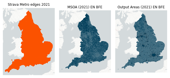
We produced results for four different geographic scopes, each shown in Figure 2, those are:
- England (Dissolved ONS Regions (December 2022) EN BFE)
- ONS Regions (December 2022) EN BFE
- Convex hulls from points for each counter source
- Convex hulls from k-means clustering of counter locations
Figure 2. Geographic scopes to intersect with Strava Metro edges and Output Areas which are the lowest level of geographical area for census statistics.
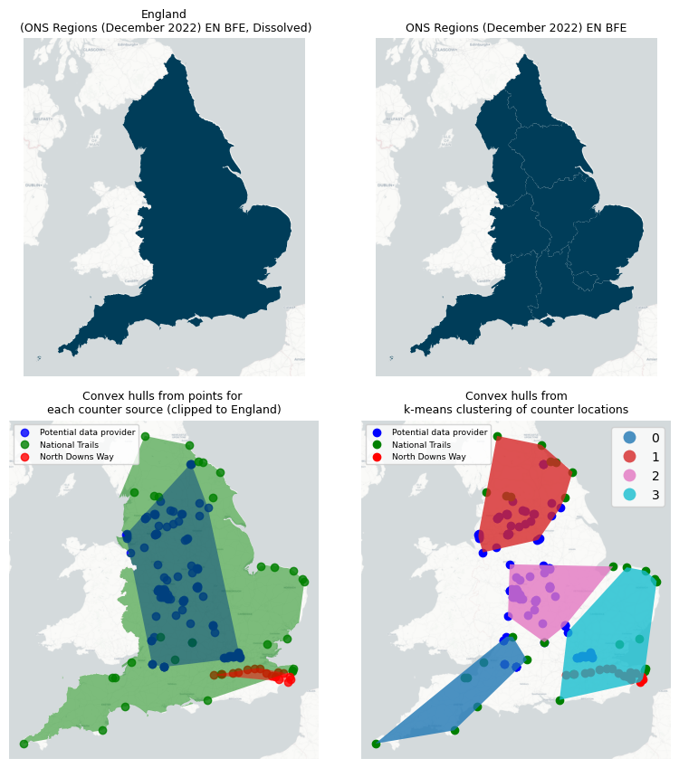
These scopes were each intersected with Metro edges, Middle Super Output Areas and Output Areas. The intersecting rows were joined to the demographic data. Comparisons could then be made for the proportion of each demographic group of interest present within each geographical scope.
Figure 3. Demographic profiles for England
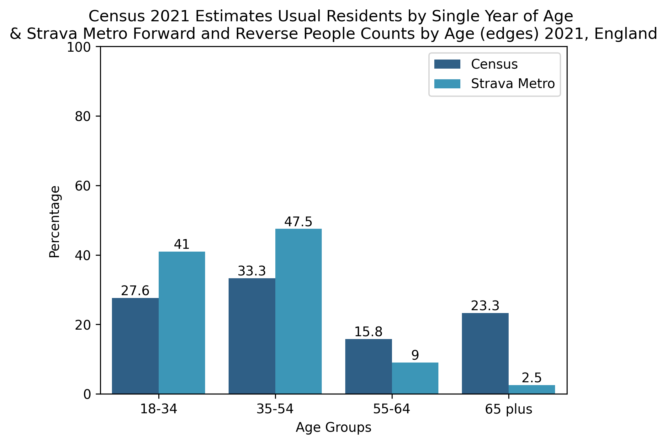
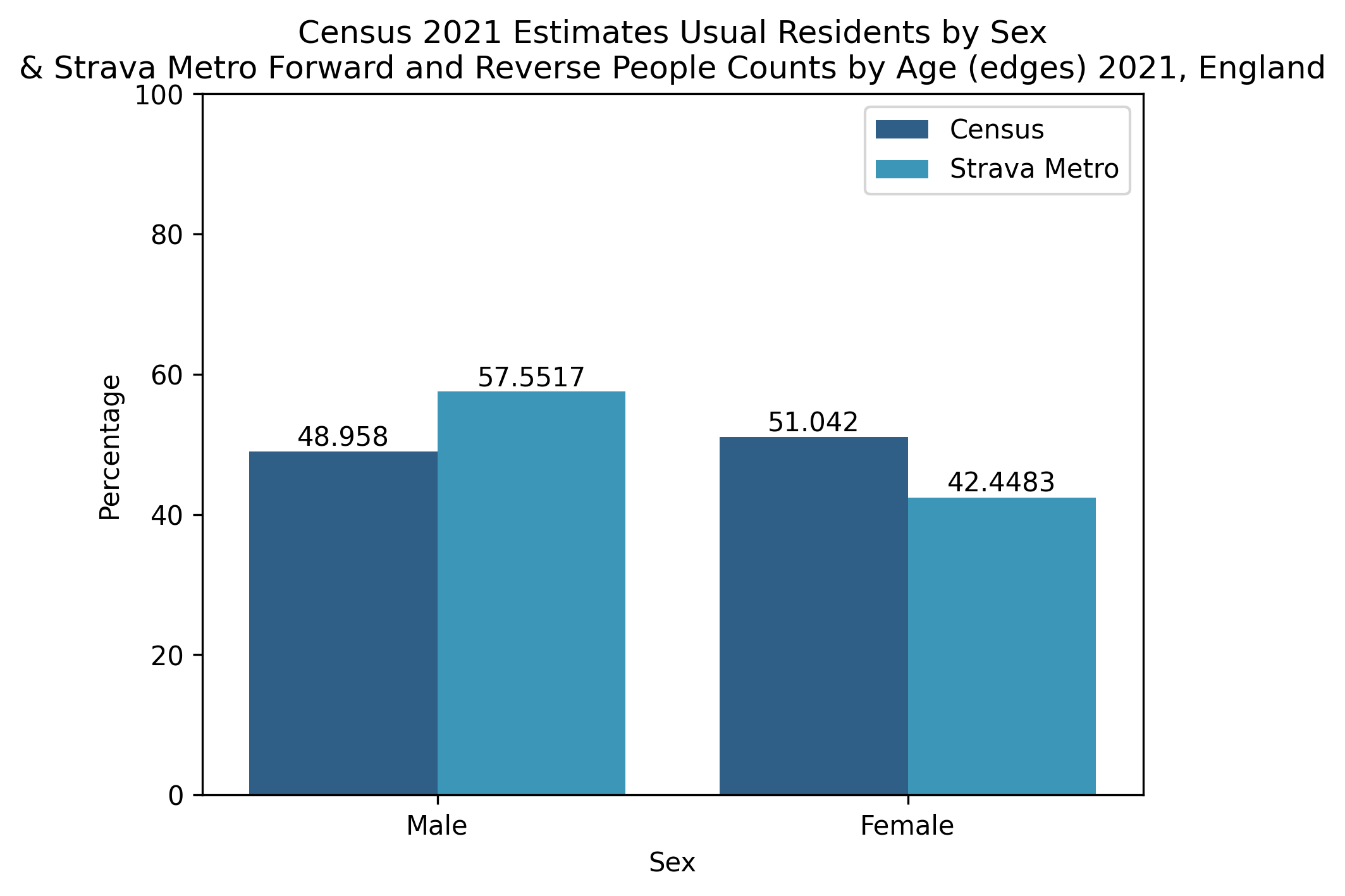
Figure 4. Demographic profiles for convex hulls from points for each counter source
Figure 5. Demographic profiles for convex hulls from k-means clustering of counter locations
Figure 6. Demographic profiles for ONS Regions
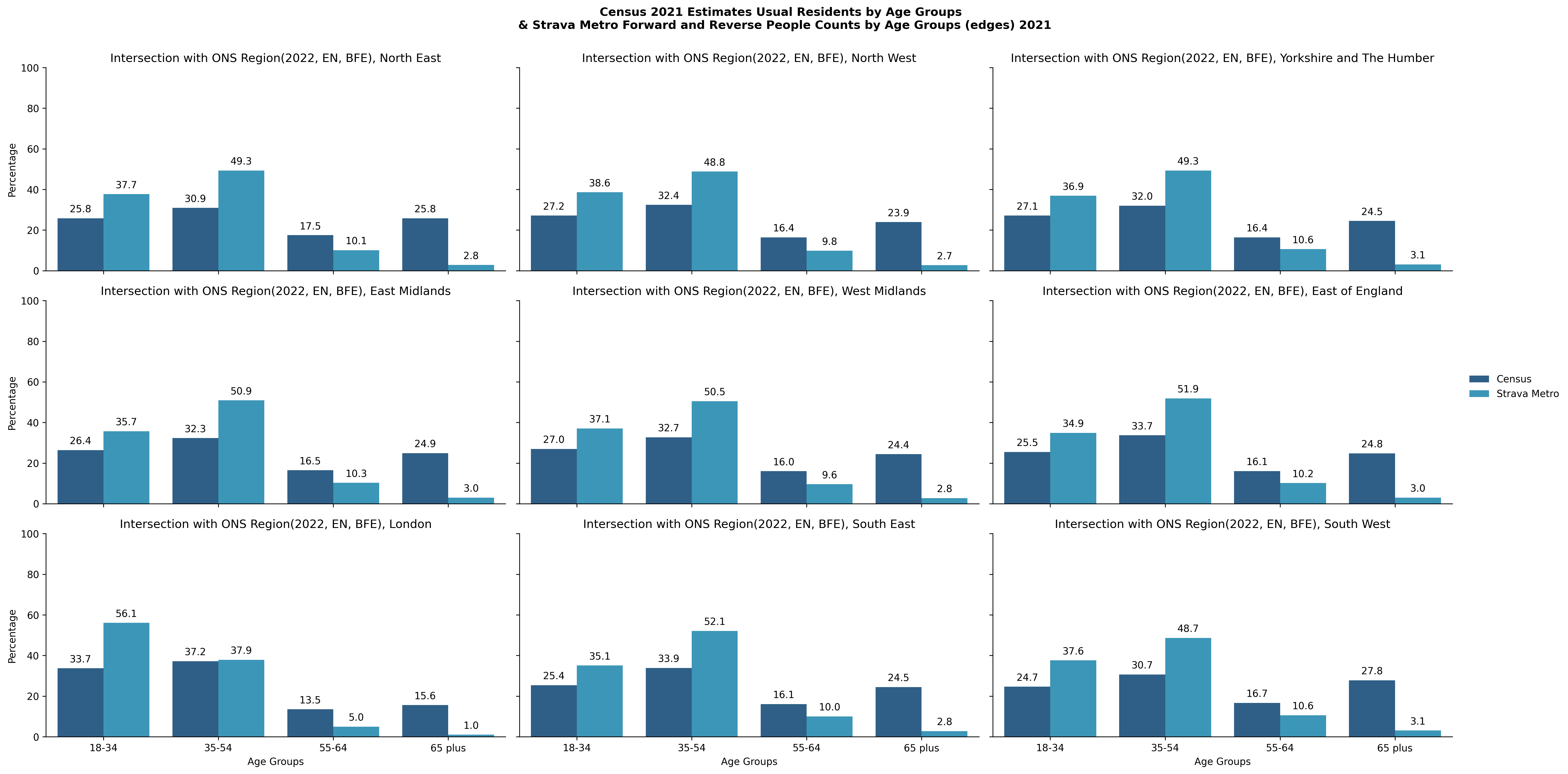
The proportion of demographic groups from the Strava Metro data and the Census 2021 datasets have been compared in Figures. 3, 4, 5, 6 for different geographical scopes. It is interesting to observe qualitatively similar patterns emerging between the two datasets for very different geographical scopes.
The Census variables are estimates for the number of people in each age and sex demographic for a given area type. The data are counts of unique individuals. The Metro data consists of rows of activity counts with unique (forward and reverse) people counts for age groups and sex. Each row represents a Metro edge with total demographic counts relative to that edge.
The sum of this data would provide the total number of edge activities and demographic counts of those edges, not the total number of Metro activities nor the demographic counts of unique individuals who completed those activities. Thus individuals and their demographic profile will have been counted for every edge included in an activity they recorded.
This means the data here are not directly comparable, however we can confirm that Strava Metro’s summaries suggest unique users by age (not shown here) do not significantly differ in proportion when compared with the results seen in the above figures (Fig 3, 4, 5, 6), except for “18-34” possessing a larger proportion and “35-54” seeing a smaller proportion. These unique user summaries cannot be published as this is against the data sharing agreement policy.
Historical weather data
Evidence from both Monitor of Engagement with the Natural Environment survey and People And Nature Survey shows weather influences people behaviour in visiting natural sites.
We use Meteostat to access open weather data from the Met Office. Specifically, we include the average monthly temperature as our variable of interest to model the impact of warmer weather on visits to natural spaces. For each counter site, we include average monthly temperature recorded at the corresponding nearest available monitoring station.
Dog Ownership
Orval Insights found that individuals that own a dog are estimated to take 3.7 times as many trips to outdoor locations as those that do not. PANS does not provide information on households that own dogs but as a proxy we used PANS published data on the location of visits and records if visitors own a dog.
Socio demographic data from Census 2011
The ORVaL insights found patterns of engagement with nature varied for different socioeconomic and demographic groups. We use the 2011 Census to gather a range of socioeconomic and demographic features for the areas around each of the people monitoring site.
Natural England spatial data on accessible green and blue space & rights of way
Natural England have carried out extensive work to produce the most comprehensive data available of accessible natural spaces in England- the Natural England Green Infrastructure Map including different type of Green and Blue infrastruture.
Amenities and points of interest
Subject matter experts in Natural England provided advice on which site amenities were related to peoples visiting behaviour. Open Street Map provides the most detailed open data on a range of amenities and points of interest across England and was used in the modelling.
Natural England’s ‘Living England’ habitat map
Examination of MENE by Hornigold and Exeter both found the land cover of a site has an impact on peoples visit behaviour. The Living England habitat probability map provides the most extensive open data on the extent and distribution of broad habitats across England, providing a valuable insight into our natural capital assets and helping to inform land management decisions.
It was developed to provide detailed habitat information to support Defra policy development and delivery. The Living England project, led by Natural England, is a multi-year programme delivering a satellite-derived national habitat layer in support of the Environmental Land Management (ELM) System and the Natural Capital and Ecosystem Assessment (NCEA) Pilot.
Rural Urban classification dataset
ORVaL Insights found participation in outdoor recreation is lower in urban residents than rural residents and to reflect this finding we used the official rural urban classification in the modelling.
After identifying the features of interest and the respective data sources, we undertake a range of pre-processing steps to prepare the features identified suitable for modelling purposes. This will be the focus of the next section.
4. Details of Feature Gathering
Our modelling approach involves estimating the monthly average people count (MAPC) to best replicate the visitor numbers from the automated people counters the approximate locations of which are shown in Figure 7.
The dataset used to train our model was a mixture of static and dynamic features. The static features were gathered by extracting features from all the static datasets mentioned above in a five-kilometre area surrounding the location of the automated people counters.
In the case of dynamic features, nearest segment of road track or similar to the corresponding people monitoring site was used to extract pedestrian Strava activity data and the nearest weather monitoring station to the respective people counter site was used for getting the weather data.
We will now illustrate the steps we have followed to prepare the identified static and dynamic predictors used for building our statistical and machine learning estimation models.
Dynamic features
People counter data
This is the variable we are trying to estimate and this feature forms the target variable for our models. The data has both spatial and temporal attributes and the location of the people counters is shown in Figure 7. Currently, we only have access to the counter data provided by Natural England and North Downs Way.
We are in conversations with another national data provider which maintains a large network of physical counters, approximate locations of those are also shown in Figure 7. The data provider can’t be named yet for commercial reasons so we will refer to them as a potential data provider.
The raw visitor count data has been cleaned after removing outliers (removing the top and bottom 10% of the data) and any missing values in the time series have been imputed using Kalman Smoother which operates on state space model. The raw and pre-processed people counter time series are shown in Figure 8 alongside the average monthly count averaged across all sites.
As shown in Figure 8, data obtained from different data providers span over slightly different time periods. For Natural England people counters, we have access to data between the period Jan-2020 – Nov-2022. On the other hand, for North Downs Way counters, we only have access to the on the ground observational count data covering the period between Sept. 2021 – Nov 2022.
Moreover, the number of spatial sites for which the monthly aggregated people counter data meet the data quality threshold is not fixed for either of the data providers. This is a data quality issue which we plan to address in the future by engaging with other data providers to gain access to a more complete on the ground people monitoring time series data.
Figure 7 A Location of people counters and the associated data providers along with number of physical sites operated by them. Figure 7 B We are in conversations with a national data provider which maintains a large network of physical counters, approximate locations of those are shown. The data provider can’t be named yet for commercial reasons so we will refer to them as a potential data provider.
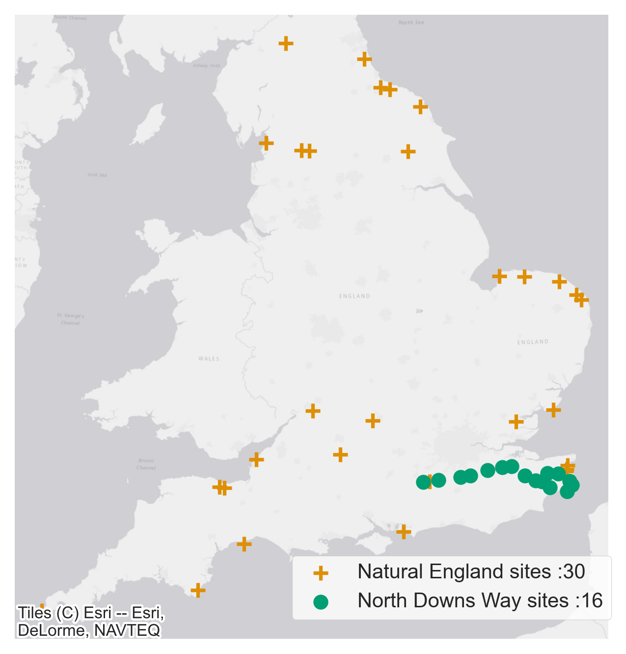
Figure 7 A
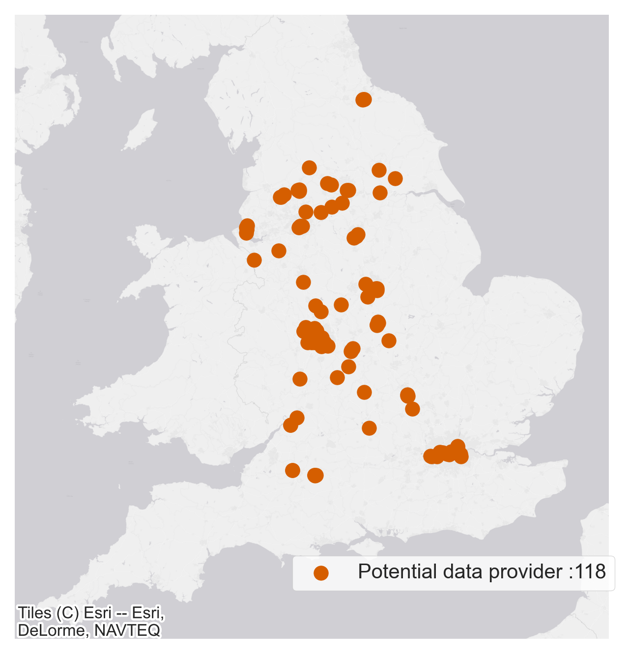
Figure 7 B
Figure 8. (a) Sample people counter location. (b) Raw and smoothed people count time series data for the sample site. (c) Monthly count averaged across all sites for each data provider.
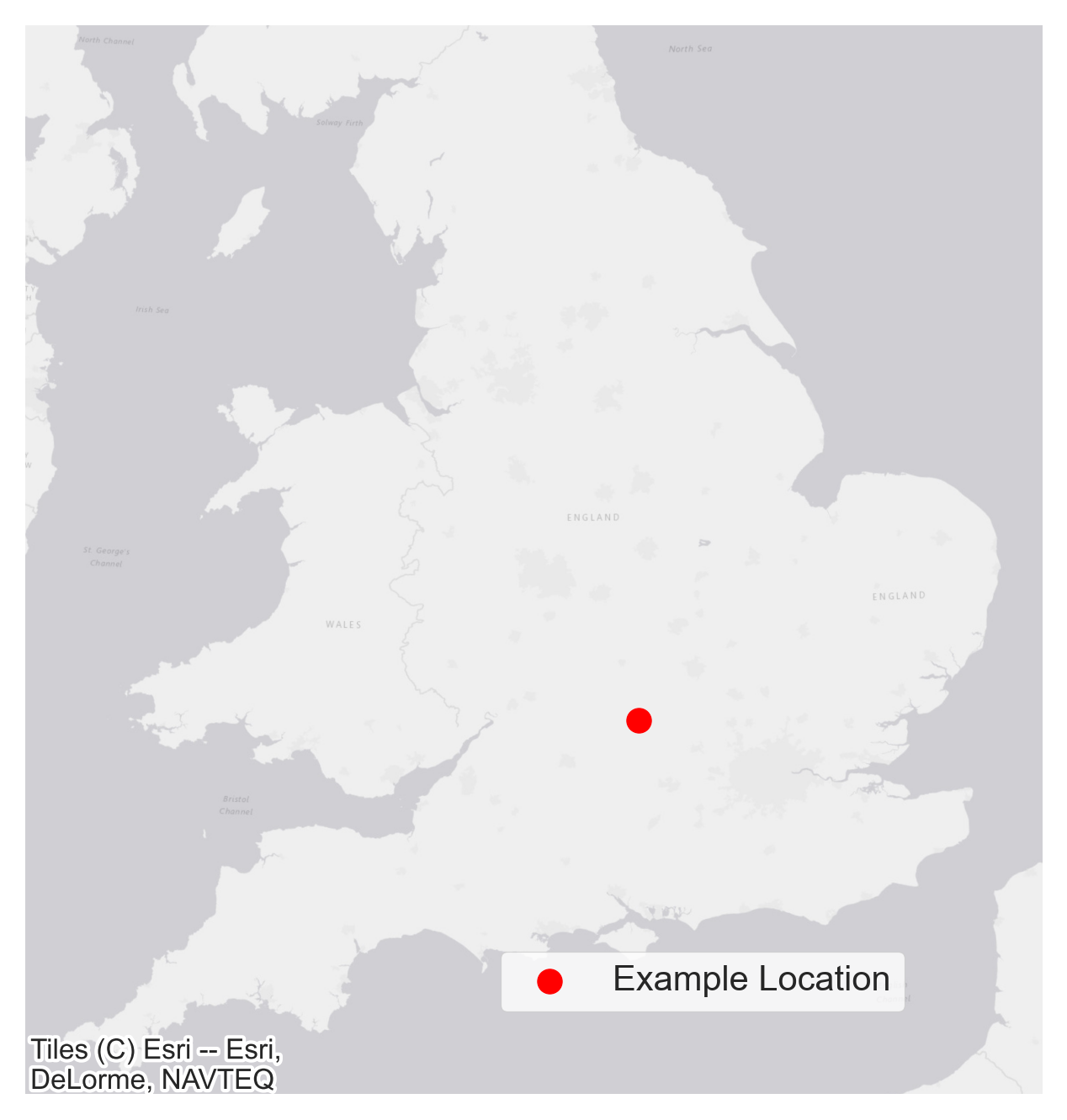
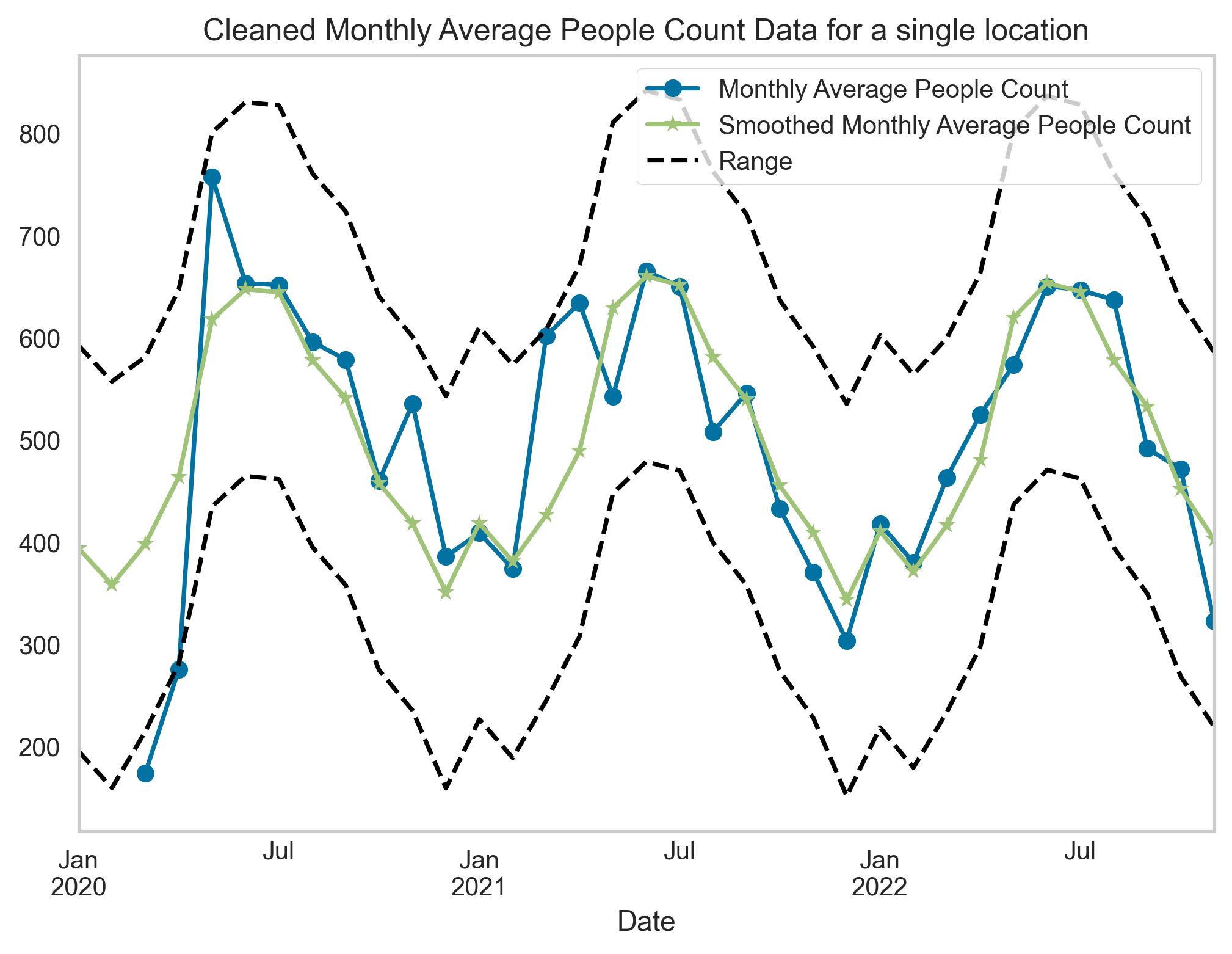
Figure 8 B
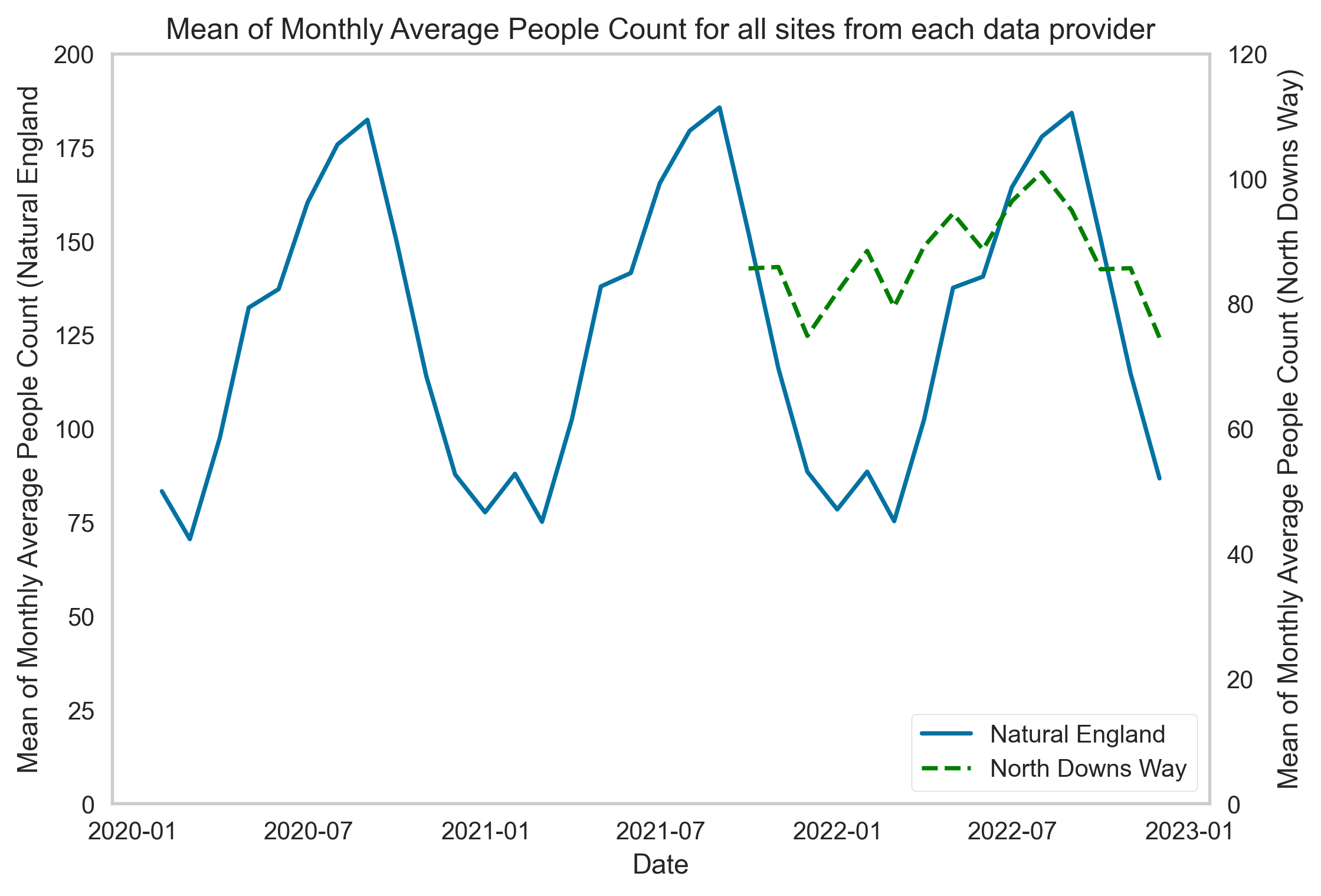
Figure 8 C
Strava Metro count data
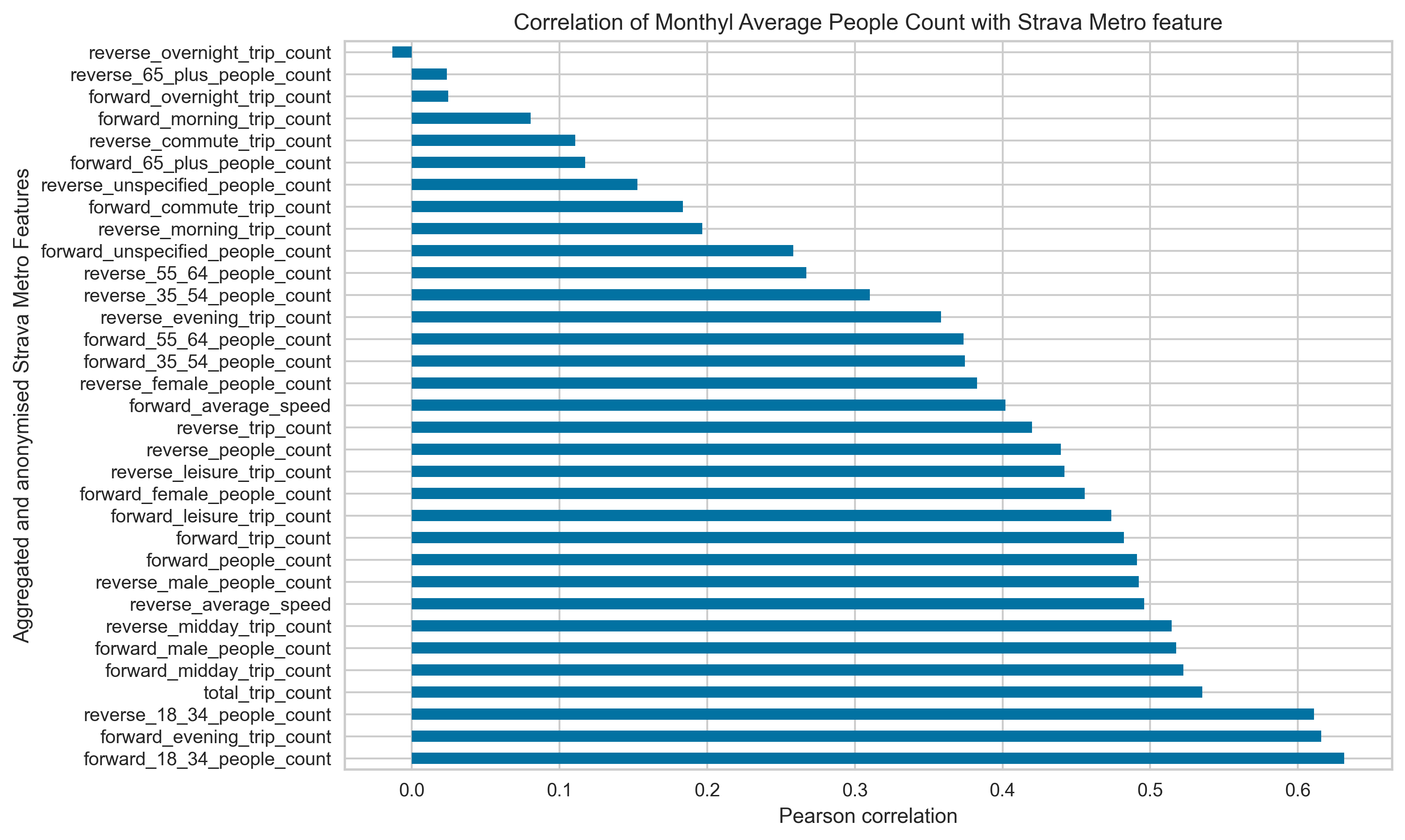
For the purposes of modelling, we focus on the Pedestrian data which includes run (including trail run), walk, and hike data combined into a single dataset. We choose total trip count as the representative feature for the Strava activities encapsulating the number of pedestrian trips on a given Strava edge (the segment of road track or similar on which user activity is recorded) during the given timeframe.
Pearson pairwise correlation between daily Strava features and daily visitation count from people counter data for all spatial sites and all time periods is shown in Figure 9.
Figure 9. Pairwise Pearson correlation between daily recorded Strava features and daily people counter data across all spatial sites January 2020 – November 2022). We choose total trip count as the representative feature for the pedestrian count based on the value of the pairwise correlation.
Historical weather features
The People and Nature Survey for England highlighted that poor or bad weather is one of the main reasons which can prohibit people from spending time in green and natural spaces. We do believe weather can play an important role in influencing visitor numbers at outside spaces and we thus include average monthly temperature to control for seasonal variations in the weather in the model.
We use Meteostat Python library which provides simple access to open weather and climate data using Pandas. Historical observations and statistics are obtained from Meteostat’s bulk data interface and consist of data provided by different public interfaces, most of which are governmental.
Meteostat focuses on historical weather and climate data that was measured on-site by weather stations around the sites of interest, we include average monthly temperature recorded at the corresponding nearest available monitoring station.
Static features
Socio-economic and demographic features
People visitation count time series dataset does not provide information on the socioeconomic and demographic profile of the visitors. We can however gather socioeconomic and demographic profile of the areas in the vicinity of the visitor monitoring sites and we address this in the following section.
As highlighted earlier, Orval Insights found that with respect to distance to home, a steep decline was observed in peoples likelihood of visiting sites further than 5km from an individual’s home. Thus, we restricted ourselves to gathering socioeconomic and demographic features within 5km buffer areas around each of the people monitoring site.
We use the 2011 Census to gather a range of socioeconomic and demographic features for the areas around each of the people monitoring site. We use the Output Areas (OAs) geometries for a finer spatial resolution of the variables of interest around the green spaces.
Output Areas (OA) provide the lowest level of geographical area for census statistics and are built from clusters of adjacent unit postcodes in the United Kingdom and are the base unit for Census data releases.
We define 5km buffer zones around the sites of interest (green spaces) and calculate the mean proportion of the following features at the OA geometries:
- Household size: 1-2 people in household**, 3+ people in household
- Age groups: Age group 0-25, Age group 25-65, Age group 65+**
- Household deprivation: Household is not deprived in any dimension **, Household is deprived in at least 1 dimension
- Employment: Economically active, Economically Inactive **, Unemployed population
- Health: Population in Good Health **, Population in Bad Health
- Ethnicity: White **, Asian/Asian British, Mixed/Black/others
- Vehicles: No cars or vans in household, 1 car or van in household **, 2 or more cars or vans in household
- Density (number of persons per square km)
One of the motivations behind focusing on the above mentioned socioeconomic and demographic features was some of the revelations in the MENE investigations highlighting some of the factors hindering people to spend more time outside in the natural world, including time-related (being too busy at work or home); health or age related; personal preferences (not interested, prefer other things), and; poor access (no suitable places, no car, safety concerns or no public transport).
Points of interest features
We engaged closely with Natural England subject matter experts on green infrastructure, access, and recreation, to identify additional datasets relevant for our investigation. Getting information on points of interest (for example amenities such as toilets) in the vicinity of natural spaces was identified as one of the important features to be included in the modelling.
OpenStreetMap (OSM) is a global collaborative (crowd-sourced) dataset and project that aims at creating a free editable map of the world containing a lot of information about our surroundings. It contains data for example about streets, buildings, different services, and land use to mention a few.
We used OSMnx a Python package to retrieve, construct, analyse, and visualise street networks from OpenStreetMap, and also retrieve data about other points of interest such as restaurants, schools, and lots of different kind of services.
We handpicked points of interests around each of the green spaces based on discussions with Natural England colleagues and independent research. Specifically, we retrieve data about the following points of interest around each people counter sites:
- amenities: bar, beer garden, bus station, cafe, coach parking, food court, holiday park, parking, restaurant, taxi station, toilets
- tourism: camp site, guest house, hotel, picnic site
- highway: bus stop
Figure 10 shows the number of points of interest expressed as a proportion of the total area of the buffer zones around each of the people monitoring sites across England. The number of people monitoring sites are uneven and thus these results need to be reported with caution.
For example, the North East region has only four visitor monitoring sites and thus has a lower total area of buffer zone when compared with the South East region for example with relatively higher number of people monitoring sites.
Figure 10(a) shows the North West, West Midlands, East Midlands and Yorkshire & the Humber regions show a high amount of all points of interest features whereas the North East, East of England, South East and South West regions have relatively low number of points of interest. Figure 10(c) shows the distribution of specifically pubs across each region.
This distribution is in contrast to that shown in Figure 10 (a) as North East, South East and South West have a higher number of pubs relative to the East Midlands and Yorkshire and Humber regions. This descriptive analysis can be useful when it comes to analysing the outputs of our machine learning model for example the significant predictors influencing the visitation count.
Figure 10. Points Of Interest features per total area of buffer zone in each region

Figure 10 a
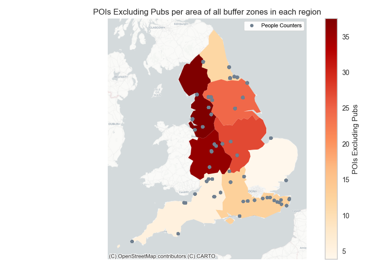
Figure 10 b
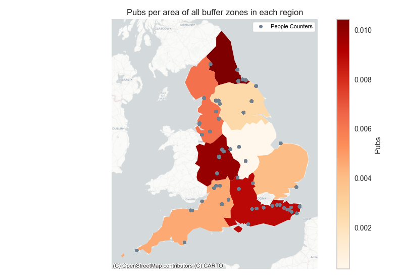
Figure 10 c
Rural Urban classification features
People monitoring sites can either be in rural or urban locations. Exploring the relationship between the site location and its respective visitation count can be of real interest and this is the motivation behind including the relevant features in the modelling.
Based on rural urban classification at the Output Area geographies, we segment 5km buffer zones around each of the counter sites into different area types. We use density based clustering on the area make up around each site to identify three land clusters shown in Figure 11. Also shown is the area make up of each identified cluster (class label). We can use these cluster labels to control for some of the area characteristics in the modelling.
Figure 11 a. Land type classification of different counter sites based on rural-urban classification at the Output Area geographies. Figure 11 b. Density based clustering to identify three land clusters and the average area falling under each cluster.
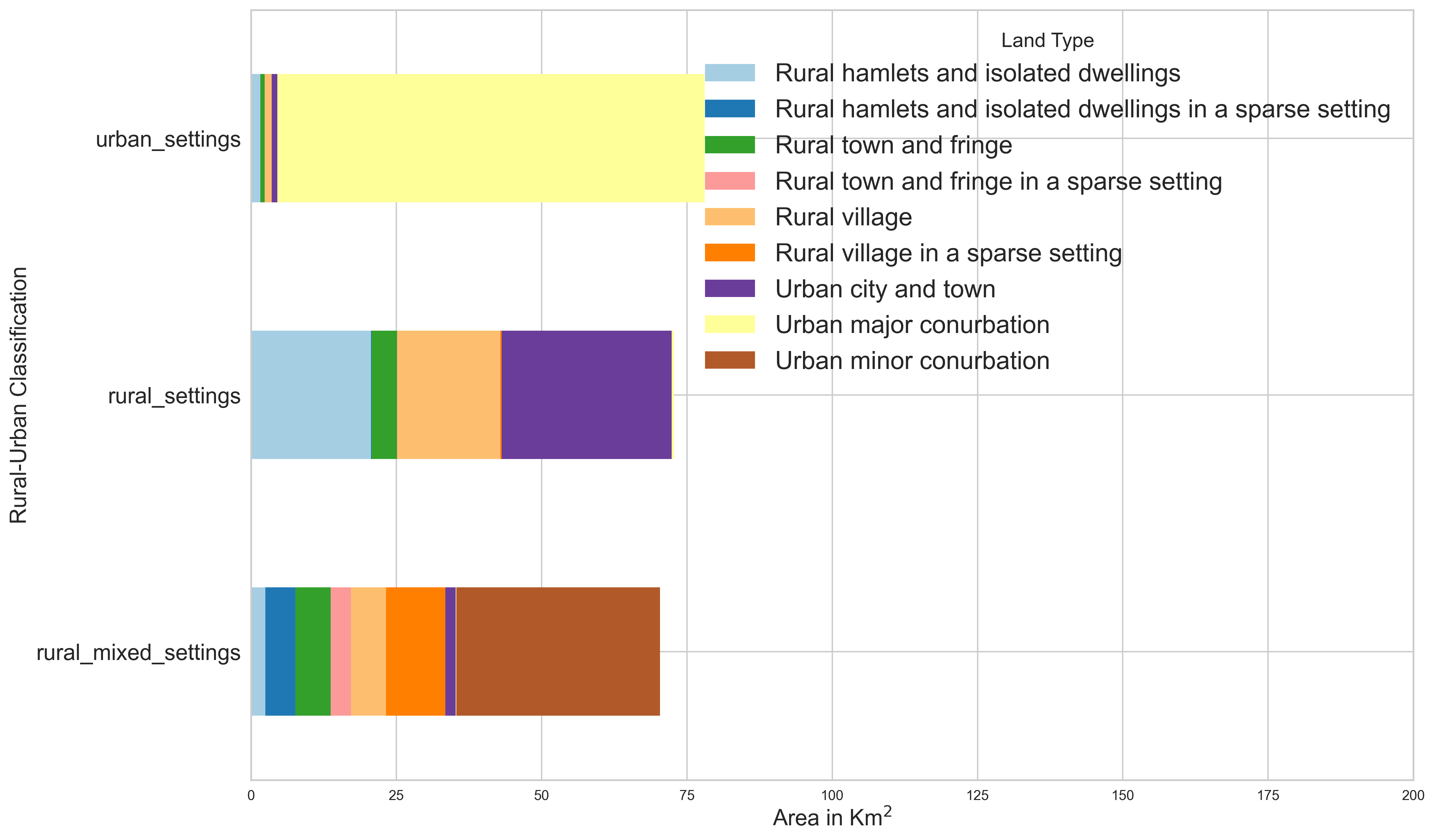
Figure 11 a
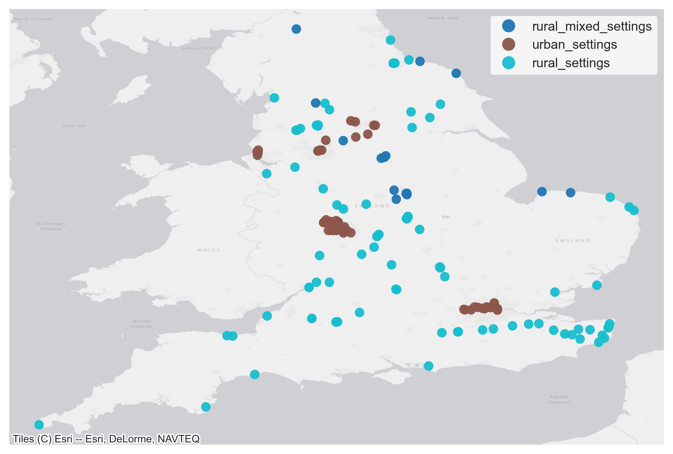
Figure 11 b
Living England Habitat Map features
Another useful feature set to be included in the modelling is the information on the extent and distribution of natural habitats in the vicinity of the people monitoring sites. The Living England habitat probability map provides such information and it shows the extent and distribution of broad habitats across England, providing a valuable insight into our natural capital assets and helping to inform land management decisions.
The Living England project, led by Natural England, is a multi-year programme delivering a satellite-derived national habitat layer in support of the Environmental Land Management (ELM) System and the Natural Capital and Ecosystem Assessment (NCEA) Pilot.
The habitat probability map displays modelled likely broad habitat classifications, trained on field surveys and earth observation data from 2021 as well as historic data layers. We use density based clustering on the area make up around each site to identify three land habitat clusters shown in Figure 12. Also shown is the area make up of each identified cluster. We can use these cluster labels to control for land habitat characteristics in the modelling.
Figure 12 a. Habitat type classification of different counter sites based on Living England Habitat Map classification. Figure 12 b. Density based clustering to identify three land habitat clusters and the average area falling under each cluster.
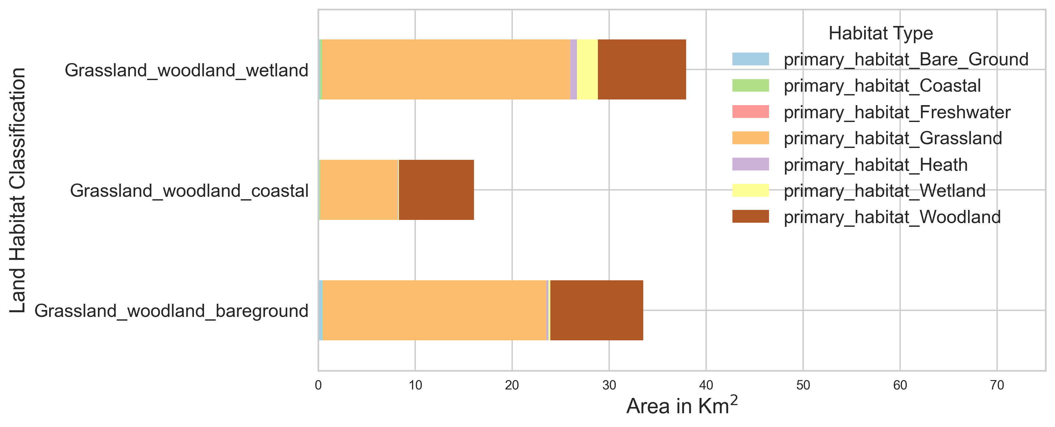
Figure 12 a
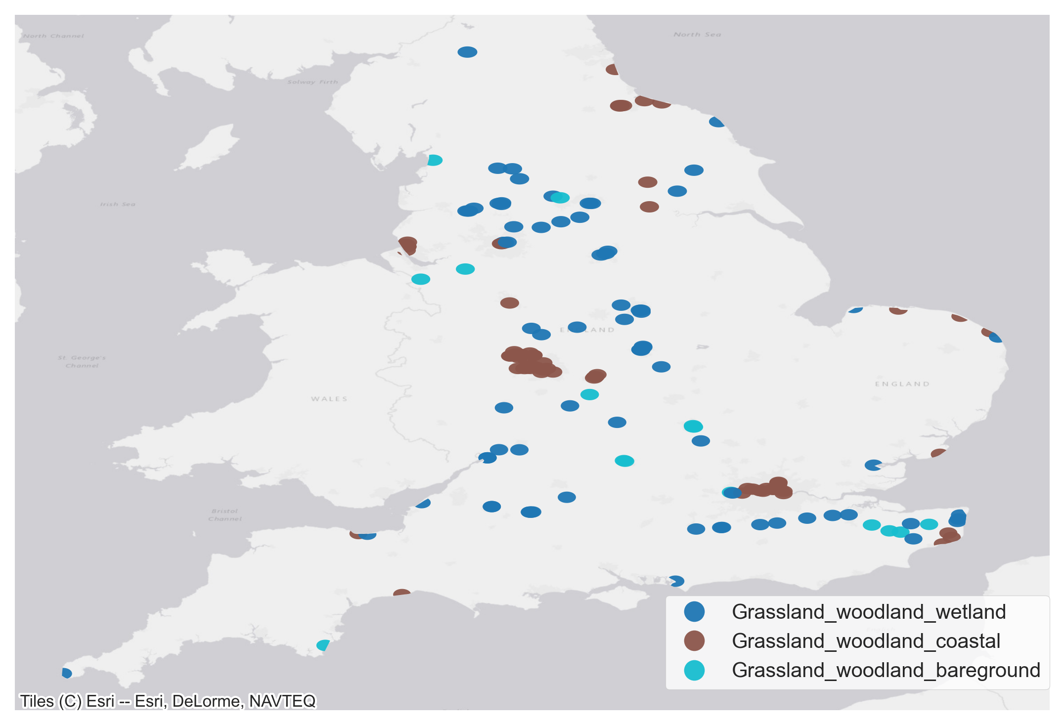
Figure 12 b
Accessible Green and Blue infrastructure features
After detailed discussions with colleagues from DEFRA and Natural England, we included additional features in the modelling to account for accessible Green and Blue spaces in the vicinity of the people monitoring sites.
We used a range of datasets to describe the location and geographical extent of different types of Green and Blue Infrastructure across England. Following extensive discussions with subject matter experts in DEFRA and Natural England, we included the following features in the modelling:
- accessible Natural Greenspace (ANG) locations: Spatial dataset describing the location and geographical extent of different types of Green Infrastructure across England, based on a systematic typology system. This includes the following accessible spaces: Access Land (CRoW), Millennium or Doorstep Green, Playing Fields, Public Park – General, Cemeteries and Religious Grounds, Play Space Provision, Public Park – Country Park, Local Nature Reserve, National Nature Reserve
- public Rights of Way ProW Density Grid (PRoW Density (m per 1km square)): This spatial dataset is a 1km grid of England showing the density of ProW each grid square
- inland waterside and ANG locations: This spatial dataset shows the geographical extent and location of inland waterside across England that intersects with the ProW network and areas of Accessible Natural Greenspace.
People and Nature Survey features
As mentioned earlier, the People and Nature Survey for England gathers evidence and trend data through an online survey relating to people’s enjoyment, access, understanding of and attitudes to the natural environment, and its contributions to wellbeing. Including relevant features from this survey can be potentially useful for our modelling purposes and model triangulation.
As pointed out earlier, one of the findings from the Survey was dog ownership was found to positively influence the likelihood of the use of natural spaces. From our modelling perspective, we approximately model dog ownership in the vicinity of the people counter sites.
We aggregate the number of visits reported in the People and Nature Survey which fall within the buffer zones around each of the people counter sites. People and Nature survey visits intersecting with the people counters locations are shown in Figure 13. We compute the average number of visits made to each people counter sites recorded in the People and Natural Survey alongside the average of all the visits made with a dog.
Figure 13 a. Location of people counters and intersection with visits reported in People and Nature Survey. Figure 12 b. Correlation between average number of visits made to people counter sites and the mean dog occupancy in the vicinity of the counter sites.
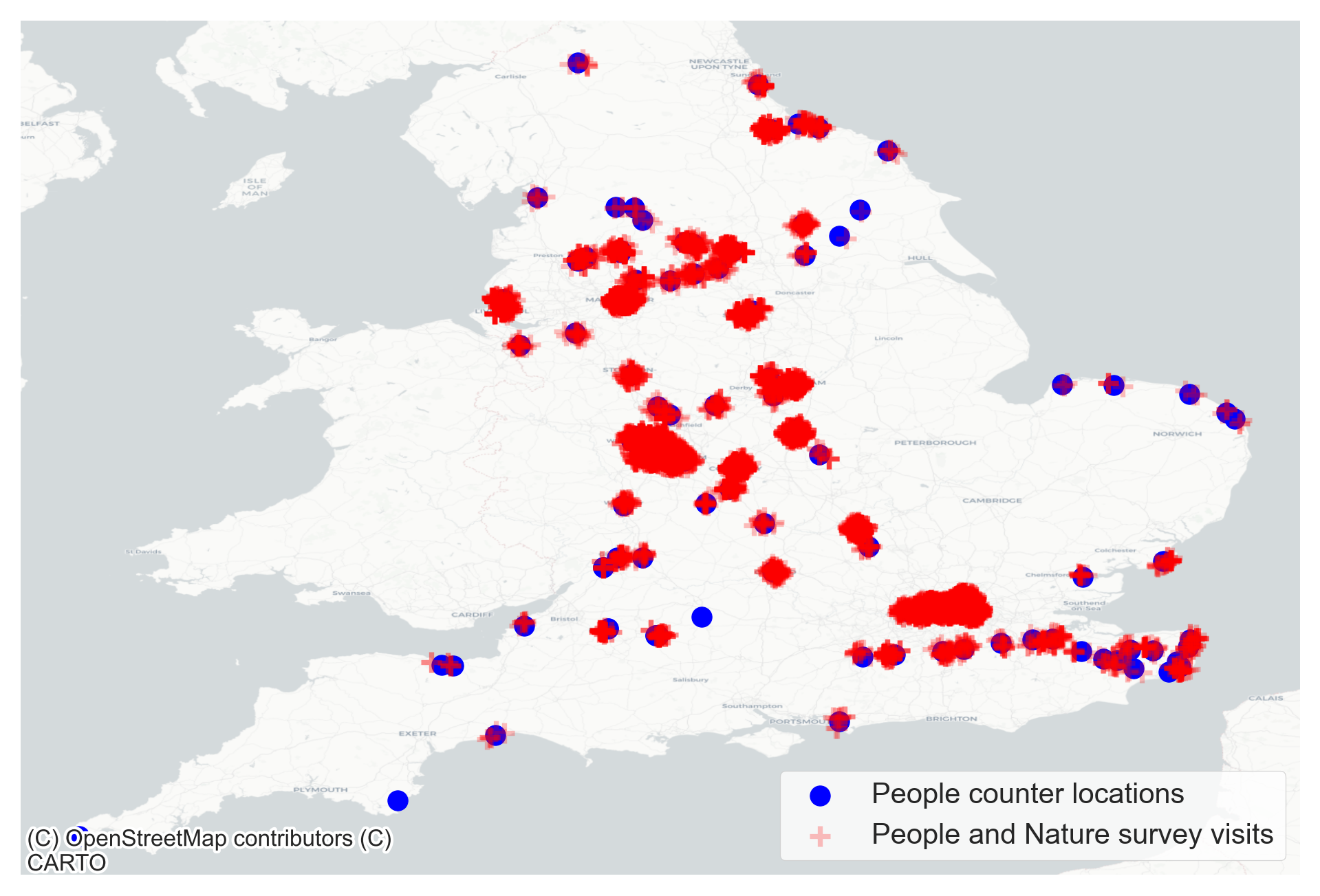
Figure 13 a
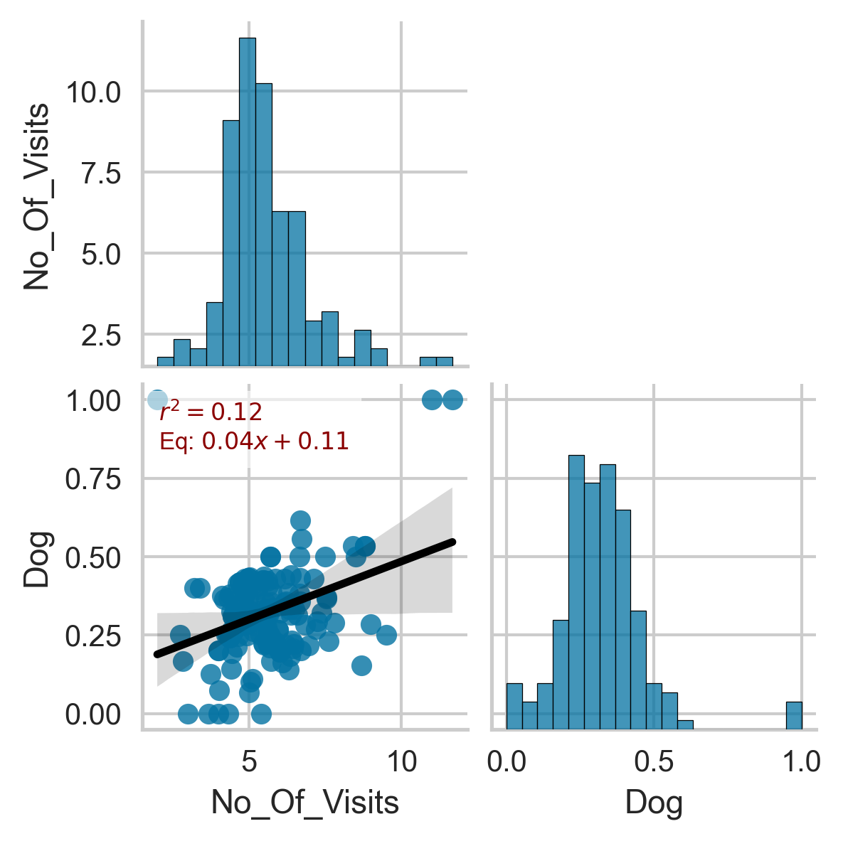
Figure 13 b
5. Feature engineering
After identifying the relevant datasets and respective features for training our statistical and machine learning models for estimating natural spaces visitation count, we made use of a few other techniques to pre-process some of the gathered features to prepare them suitable for modelling.
We start with using exploratory factor analysis to account for spatial correlation amongst the demographic features. We then compute Pearson pairwise correlation to remove other highly correlated features. We also combine some of the categorical features to avoid the problem of class imbalance.
Lastly, we compute the variance inflation factor scores to sequentially drop other highly correlated features. These are explained in detail in sections below.
Exploratory factor analysis for features with spatial overlap: demographic features
We start with removing the baseline features from the feature list. We then employed exploratory factor analysis (EFA) on our input features to understand the correlation amongst the features and help understand some of the influences of the visitation count as explained later.
EFA is a statistical method to reduce dimensionality of our features through estimating the minimum number of unobserved factors that represent the observed variables. In other words, EFA describes variability among observed correlated variables in terms of a potentially lower number of unobserved variables called factors.
In our case, we use EFA to evaluate the interaction between our features and decide how to account for those as inputs to our model. To formulate, we consider each observable variable (factor indicator) Xi as a linear function of independent factors and error terms which can be written as \(\)
$$ \begin{equation}
X_{i}=\zeta_{i0}+\sum_{k}\zeta_{ik}F_{k}+e_{i}
\end{equation} $$
In the equation above ζi0 is the bias term and the error terms ei, serve to indicate that the hypothesised relationships are not exact. In the vocabulary of factor analysis, the parameters ζik is referred to as factor loading of variable Xi on factor Fk. It can be shown that the variance of Xi consists of two parts
$$ \begin{equation}
{\rm var}(X_{i})=\underbrace{\zeta_{i1}^{2}+\zeta_{i2}^{2}…}_\text{communality}+\sigma_{i}^{2}
\end{equation} $$
The first part, the communality of the variable, is the part that is explained by the common factors Fk(k = 1,2,…N). The second part, the specific variance, is the part of the variance of Xi that is not accounted for by the common factors. One of the prime goals in exploratory factor analysis is to determine a set of loadings which bring the estimate of the total communality as close as possible to the total of the observed variances.
To perform EFAs on our dataset, we use Python’s FactorAnalyzer package. We choose a loading threshold of 0.5 to obtain the features contributing most to each individual factor. Factor analysis allowed us to gain invaluable insights into the dataset and account for interactions amongst some of the predictors identified to be used in the model.
Table 1 shows the factor loadings from EFA; we have only reported those with absolute loading cut-off greater than 0.5. Factors in essence represent common communality across features and the associated factor loadings show the extent to which each feature has contributed to each factor.
This means the features with large absolute factor loadings for each factor tend to correlate with each other and the associated factor can represent their interrelations. For instance, in our analysis below, we can see relatively large factor loadings for the first factor for Proportion of households with no cars or vans and density features.
This shows strong correlation amongst these features suggesting spatial overlap between areas with higher proportion of households with no access to private transport and more densely populated areas. We will make use of the results of EFA to obtain useful insights into the important factors influencing the visitor numbers to outside spaces.
Table 1. Results of exploratory factor analysis of the static features where − is used to indicate the respective factor loading is below the chosen threshold of 0.5.
| Factor_1 Factor_2 Factor_3 | |||
| 3+ people in household | – – 1.15 | ||
| Age group 0-25 | – – 0.65 | ||
| Age group 25-65 | 0.76 -0.67 – | ||
| Household is deprived in at least 1 dimension | – | 0.75 | – |
| Economically active | – | -1.03 | – |
| Unemployed_population | – | 0.61 | – |
| Population in Bad Health | – | 0.92 | – |
| Asian/Asian British | – | – | 0.75 |
| … 2 or more cars or vans in household | -0.81 | – | – |
| Density (number of persons per sq_km) | 1.04 | – | – |
Pearson pairwise correlation for variable reduction: points of interest features
We compute the density of the chosen points of interests (per square km) falling within the buffer zones around the people counter sites and we use these normalised features in the modelling.
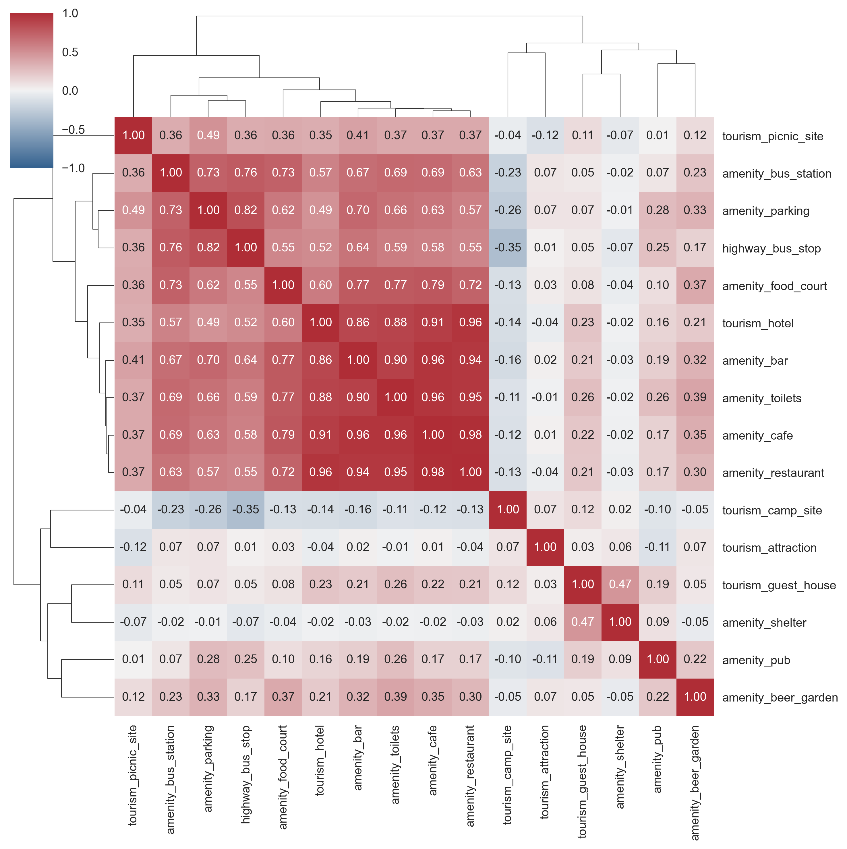
Since some of chosen points of interests are expected to be spatially correlated with others, we can compute pairwise Pearson’s correlation amongst the chosen variables to explore this correlation in a bit more detail and the result is shown in Figure 14. We can easily confirm that a high degree of correlation exists amongst a subset of features.
For example, the following points of interest have high degree of pairwise correlation: amenity (bar), amenity (cafe), amenity (restaurant), amenity (hotel) and tourism (hotel) (possibly indicating higher likelihood of these amenities existing together in dense urbanised areas). We make use of these results to remove those points of interest features with high degree of pairwise correlation.
Figure 14. Pairwise Pearson correlation amongst the different Points of interest features is shown through a hierarchically-clustered heatmap.
Variable amalgamation to deal with Class imbalance: area type and habitat type features
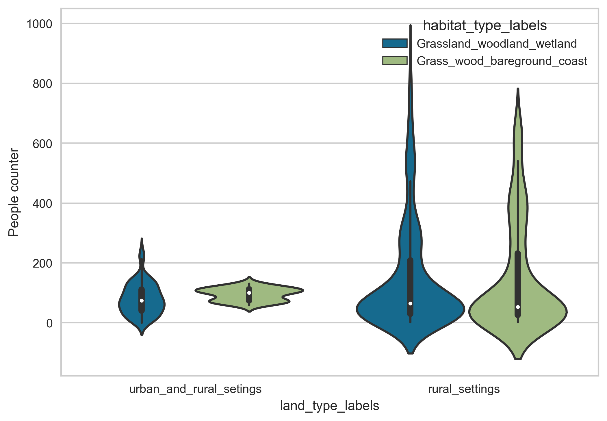
Using density-based clustering we classified each individual green space into distinct classes based on land type and habitat types. Majority of the green spaces are classified in rural settings and classed under Grassland-woodland-wetland habitat type and have thus been fixed as reference categories for modelling purposes.
As mentioned earlier, currently We thus encounter a situation where we have class imbalance in our training data where we do not have proportional representation from all land type and habitat type labels.
For example, in the training dataset (with observation count available) the count of different spatial sites assigned to habitat labels looks as follow: Grassland-woodland-wetland: 23; Grassland-woodland-coastal: 6; Grassland-woodland-bare ground: 6. Similarly, the count of different spatial sites assigned to land type labels looks as follow: rural-settings: 30; rural-mixed-settings: 5; urban-settings: 0.
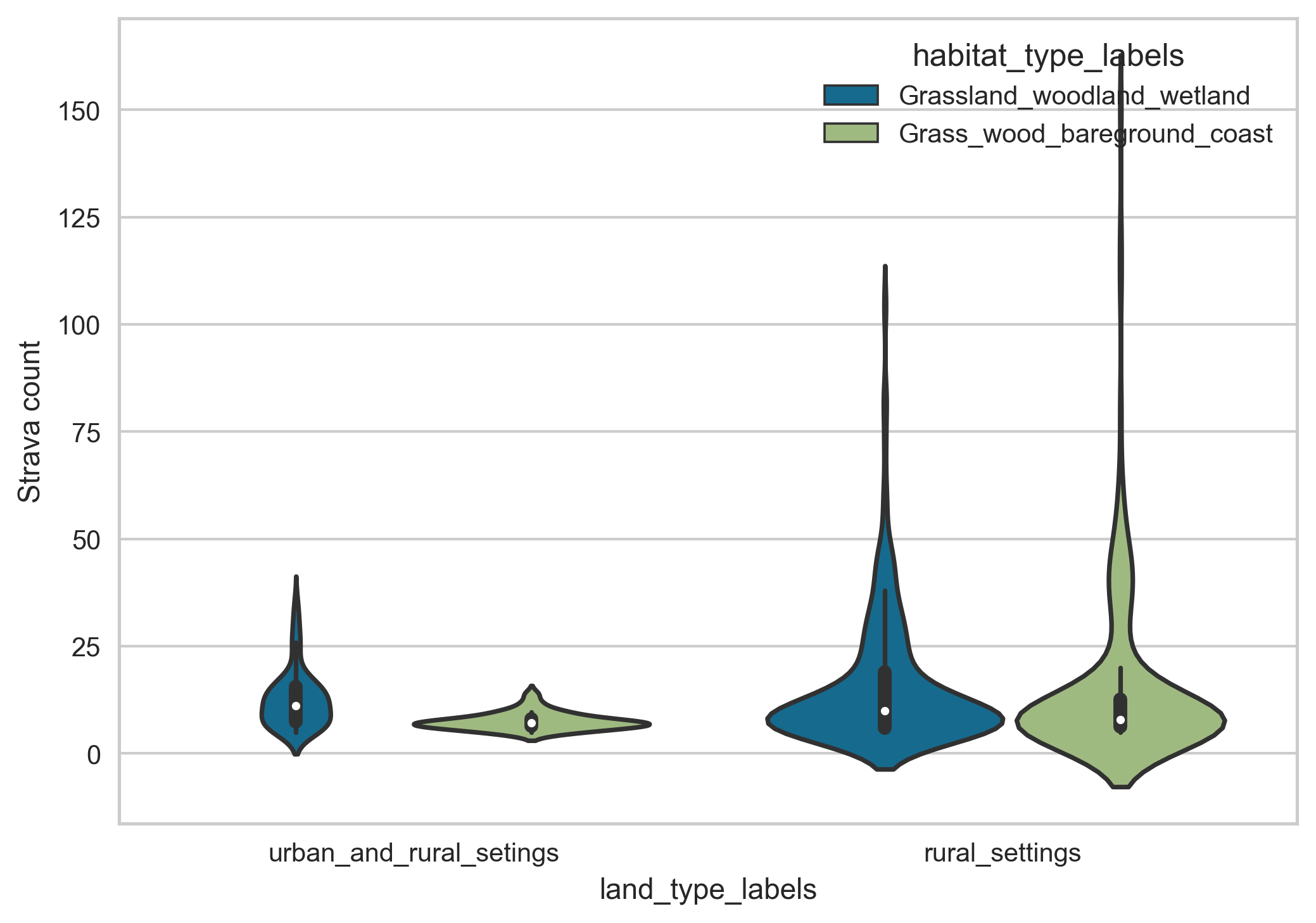
To deal with this issue, we combine the two lowest minority classes together to avoid some of the issues with class imbalance in the data. The distribution of the people counter time series data and corresponding Strava activity data labelled under these revised land habitat and land type classes is shown in Figure 15.
Figure 15. The distribution of the people counter time series data (Top) and corresponding Strava activity data (Bottom) classed under the land type and habitat type classes.
Variance inflation factor to remove inter-variable correlations
We have gathered a range of static and dynamic predictors to accurately estimate the visitor numbers for a set of spatial locations across England. As illustrated in the previous sections, we do not expect all these predictors to be completely independent of each other.
Although, we have taken steps to account for spatial interaction amongst some of the features and removing highly correlated variables within a given dataset, we still have to address possible inter-variable correlation coming from different datasets to avoid the issue of multicollinearity.
The Variance Inflation Factor (VIF) is a measure of collinearity among correlated variables. We choose a VIF score threshold of 10 and sequentially drop features which fail to meet this criterion.
VIF score of all the variables initially present in our variable list and those which meet the threshold criterion is shown in Table 2. Based on this selection, our chosen variables to be used in the modelling stage are shown in Table 3.
Table 2.(a) VIF score of all the variables initially present in our feature list
| Features | VIF Factor |
| amenity shelter | 1.65 |
| tourism attraction | 1.65 |
| amenity beer garden | 2.16 |
| tourism camp site | 2.44 |
| amenity pub | 2.53 |
| tourism guest house | 3.67 |
| tourism picnic site | 4.04 |
| amenity food court | 5.71 |
| amenity bus station | 8.07 |
| Asian/Asian British | 20.12 |
| amenity parking | 22.68 |
| highway bus stop | 28.14 |
| Mixed/Black/others | 32.60 |
| amenity toilets | 53.98 |
| amenity bar | 69.19 |
| Unemployed population | 76.06 |
| tourism hotel | 98.45 |
| Density (number of persons per sq km) | 123.76 |
| 2 or more cars or vans in household | 246.85 |
| amenity cafe | 306.28 |
| Population in Bad Health | 358.95 |
| Age group 0-25 | 624.94 |
| No cars or vans in household | 643.80 |
| amenity restaurant | 651.53 |
| 3+ people in household | 710.40 |
| Household is deprived in at least 1 dimension | 906.32 |
| Economically active | 3182.56 |
| Age group 25-65 | 4377.06 |
Table 2.(b) The final VIF score of variables remaining after sequential removal of variables with high VIF factor scores.
| Features | VIF Factor | |
| tourism attraction | 1.10 | |
| amenity shelter | 1.37 | |
| tourism camp site | 1.42 | |
| amenity beer garden | 1.45 | |
| amenity pub | 1.80 | |
| tourism picnic site | 1.92 | |
| tourism guest house | 1.95 | |
| tourism hotel | 2.07 | |
| Asian/Asian British | 2.12 | |
| 2 or more cars or vans in household | 2.13 | |
| amenity food court | 2.27 | |
Table 3. List of static and dynamic features used for modelling natural spaces visitation count.
| Dataset | Features | Temporal |
| Strava Metro | total trip count | Dynamic |
| Weather | tavg (monthly average temperature) | Dynamic |
| Socioeconomic and demographic data | Asian/Asian British, Density (number of persons per sq km), 2 or more cars or vans in household.
|
Static |
| Green and Blue infrastructure | Accessible blue space area | Static |
| Open Street Map | Points of interest features: tourism camp site, tourism guest house, highway bus stop, tourism attraction, amenity pub, amenity beer garden, amenity bus station, amenity food court, amenity shelter. | Static |
| Rural Urban classification | rural and urban mixed settings
|
Static |
| Lanh habitat classification | Grassland woodland bare ground coast | Static |
| People and Nature Survey | Mean dog occupancy in the vicinity of each people monitoring site. | Static |
6. Modelling approaches
Our prime goal in this work is to use new approaches to estimate the number of visitors using the natural spaces.
To achieve this, we have gathered a range of features as outlined in the previous sections. However, some of the features are static for example. By definition, they do not change over the modelling time while others are non-static or dynamic and they do change over time.
Strava activity data and weather data are the two dynamic predictors we plan to include to model our target variable which is the people visitation counts. Since the timescales of variation of the static and dynamic predictors are different, we use these predictors in two different ways to model our target variable.
Separation of static and dynamic predictors: Panel data structure and Fixed effects model
One of the difficulties we have is that despite introducing a range of predictors to account for spatial-temporal characteristics of the natural spaces, it is not obvious that the relationship between all the predictors and the target variable is causal or not.
It could be that certain natural sites say in the South tend to get warmer weather and also attract more visitors. This confounder is not something we can measure in its entirety. For instance, natural beauty of a site is a difficult attribute to capture. This can potentially introduce omitted variable bias in the modelling.
The methodology used for this section is based on the techniques presented but in short since quantifying all physical attributes of a spatial site is not possible we make use of panel data structure of our time series data and fixed effects model approach to solve this problem.
Panel data is a dataset with repeated observations of the same unit (natural sites in our case) over multiple periods of time. We track each site over an extensive period (January 2020 to November 2022).
Weather, Strava activity count and the number of visitors (the outcome) change over time. Spatial attributes of a site, the unmeasured confounder, roughly stays the same over the entire time period of interest.
When estimating the effect of weather on visitor numbers we introduce a dummy variable for each site in our regression model, regression finds the effect of weather while keeping the site variable fixed. Adding this dummy to control for all fixed site attributes is what we refer to as a fixed effect model.
It can be easily shown that using panel data with a fixed effect model is as simple as adding a dummy for the (time-fixed) entities. However, it is not practical to introduce dummy variables for each individual entity (site) especially when the number of entities can be arbitrary large.
Instead, we can use the fact that running a regression on a dummy variable is as simple as estimating the mean for that dummy. Furthermore, it can be shown that one can de-mean the outcome and predictor variables to remove all variables that are constant across time and this happens identically for both observed and unobserved variables.
One is thus able to use fixed effect model to eliminate all (fixed over time) omitted variable biases from the model. Following de-meaning of the data, we can properly evaluate the effect of the dynamic predictors on the outcome variable after accounting for fixed observed and unobserved variables.
Influence of weather
We follow the recipe outlined in the previous section and explore the influence of weather on the number of visitors in outside spaces. The analysis assumes weather (monthly average temperature) is the only dynamic influence affecting the observational time series people count and model to remove site-specific static attributes.
The results are shown in Table 4. The analysis based on fixed effects model approach is telling us that on average, a one unit increase in temperature leads to 6.58 unit increase in the number of visitors.
Table 4. Fixed effect model approach to eliminate all omitted variable bias from the model and estimate the effect of weather on the number of visitors visiting outside natural spaces.
| coef | std err | t | P>|t| | [0.025 | 0.975] | |
| Intercept | 0 | 2.301 | 0 | 1.0 | -4.515 | 4.515 |
| tavg | 6.580 | 0.519 | 12.690 | 0.000 | 5.562 | 7.598 |
As the seasonal patterns and average monthly temperature are correlated features, we can also look at the effect of weather for each individual seasons separately. This is shown in Table 5 and it confirms that average monthly temperature is a positive predictor of visitor numbers in all seasons except Winter over which the temperature effect is not found to be significant.
Table 5. Shown here are the non-standardised regression coefficients for separate regression models for each season. For each season, we use a fixed effects approach and control for sites’ specific (static) attributes.
| Fixed effects model for winter | coef | std err | t | P>|t| | [0.025 | 0.975] |
| Intercept | 0 | 1.566 | 0 | 1.0 | -3.087 | 3.087 |
| tavg (average temperature) | -0.3132 | 1.325 | -0.236 | 0.813 | -2.926 | 2.299 |
| Fixed effects model for spring | coef | std err | t | P>|t| | [0.025 | 0.975] |
| Intercept | 0 | 2.037 | 0 | 1.0 | -4.014 | 4.014 |
| tavg | 2.9458 | 0.712 | 4.139 | 0.0 | 1.543 | 4.349 |
| Fixed effects model for summer | coef | std err | t | P>|t| | [0.025 | 0.975] |
| Intercept | 0 | 2.307 | 0 | 1.0 | -4.548 | 4.548 |
| tavg | 6.2764 | 1.424 | 4.407 | 0.0 | 3.469 | 9.084 |
| Fixed effects model for autumn | coef | std err | t | P>|t| | [0.025 | 0.975] |
| Intercept | 0 | 2.390 | 0 | 1.0 | -4.712 | 4.712 |
| tavg | 4.5290 | 0.980 | 4.622 | 0.0 | 2.597 | 6.461 |
The coefficients reported in Table 4, Table 5 signifies how much the mean of the dependent variable (visitor count) changes given a one-unit shift in the independent variable while holding other variables in the model constant.
These are useful results and allow us to infer an (average) relationship between the predictor(s) and the outcome variable. In addition to looking at this average relationship, one can also address the effect of the chosen dynamic variable on the visitor’s count for each individual site separately.
We have explored this and have uncovered regional dependence of visitation counts. However, because of limited training data currently available to us and incomplete time series people counts for certain sites we will revisit this in a future investigation.
Influence of Strava count and weather
We again make use of fixed effects model approach to control for all static attributes across all people monitoring sites. We build a regression model on the only dynamic variables after de-meaning the data and thereby controlling for all sites’ specific static attributes.
The results are shown in Table 6. We find both the dynamic predictors have statistically significant and positive regression coefficients. It is worth reporting that the resulting residuals are not completely randomly distributed, and we believe the analysis can further benefit from spatial segmentation and using a multi-group approach which we plan to explore in a future investigation.
Table 6. We regress the visitor numbers against the average monthly temperature for each site and the corresponding Strava activity count.
| Fixed effects model | coef | std err | t | P>|t| | [0.025 | 0.975] |
| Intercept | 0 | 2.202 | 0 | 1.0 | -4.323 | 4.323 |
| total trip count | 1.7447 | 0.198 | 8.814 | 0.000 | 1.356 | 2.133 |
| tavg | 5.9483 | 0.502 | 11.860 | 0.000 | 4.964 | 6.933 |
Combining static and dynamic predictors: Machine learning approach
We next follow a machine learning approach to address the problem of estimating visitor numbers based on the identified static and dynamic predictors. We follow the following steps in the model development:
Unlike the previous sections, we do not separate the static and dynamic predictors identified in Table 3 and use both the static and dynamic features collectively to estimate our target variable. In a future investigation, we plan to compare the present approach with a two-way fixed effect approach. This involves two modelling steps: a) modelling visitation count only on the static features and b) estimating the impact of changes in dynamic features on those in residuals from step (a) (for example the remaining effects after removing those from static features). Estimating the residuals by dynamic features can be incorporated under a linear or non-linear approximation including through use of machine learning techniques. This approach can facilitate both estimation of visitation counts in diverse spatial locations and inferences of the main influences of the visitation counts.
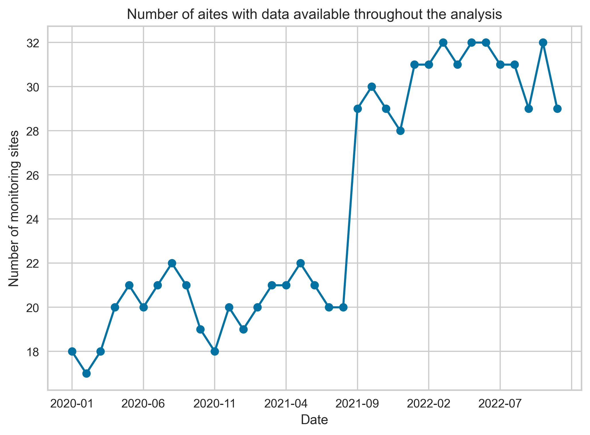
We note that the number of spatial sites for which we have been able to assemble all the predictors and the outcome variable is not constant over the time period between January 2020 to November 2022. This is reflected in Figure 16
Figure 16. Temporal variation in the number of counter sites present in the collated dataset.
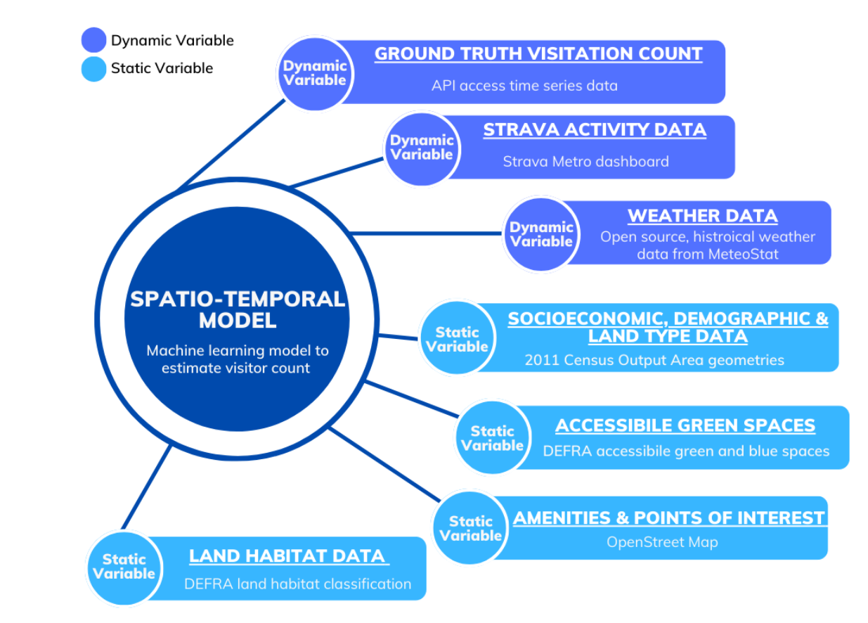
We follow a data augmentation approach and combine the static and dynamic predictors for all spatial sites and develop a spatial-temporal model to estimate visitor numbers in natural spaces as shown in Figure 17.
Although, we do not have access to the ground truth data from a potential data provider people monitoring network but we make use of the counter locations from all data providers to gather relevant static and dynamic features for the model.
Figure 17. A list of different dynamic and static variables combined to develop a spatio-temporal model to estimate Monthly Average People Count.
We split the dataset into train and test subsets in a stratified fashion using sites as class labels. We fit an estimator using the dynamic and static predictors on the train dataset. We start with an ordinary least square estimator to model the monthly aggregated visitor count at diverse spatial locations.
Following the training, we use the fitted model to estimate visitor numbers on unseen test data. We also apply regularisation to tackle the issue of potential overfitting and feature selection in the training step.
In the anticipation of future access to a more diverse training data, we make use of an automated machine learning workflow to develop an ensemble estimator which combine the predictions of several base estimators to improve generalisability and robustness over a single estimator.
Outputs
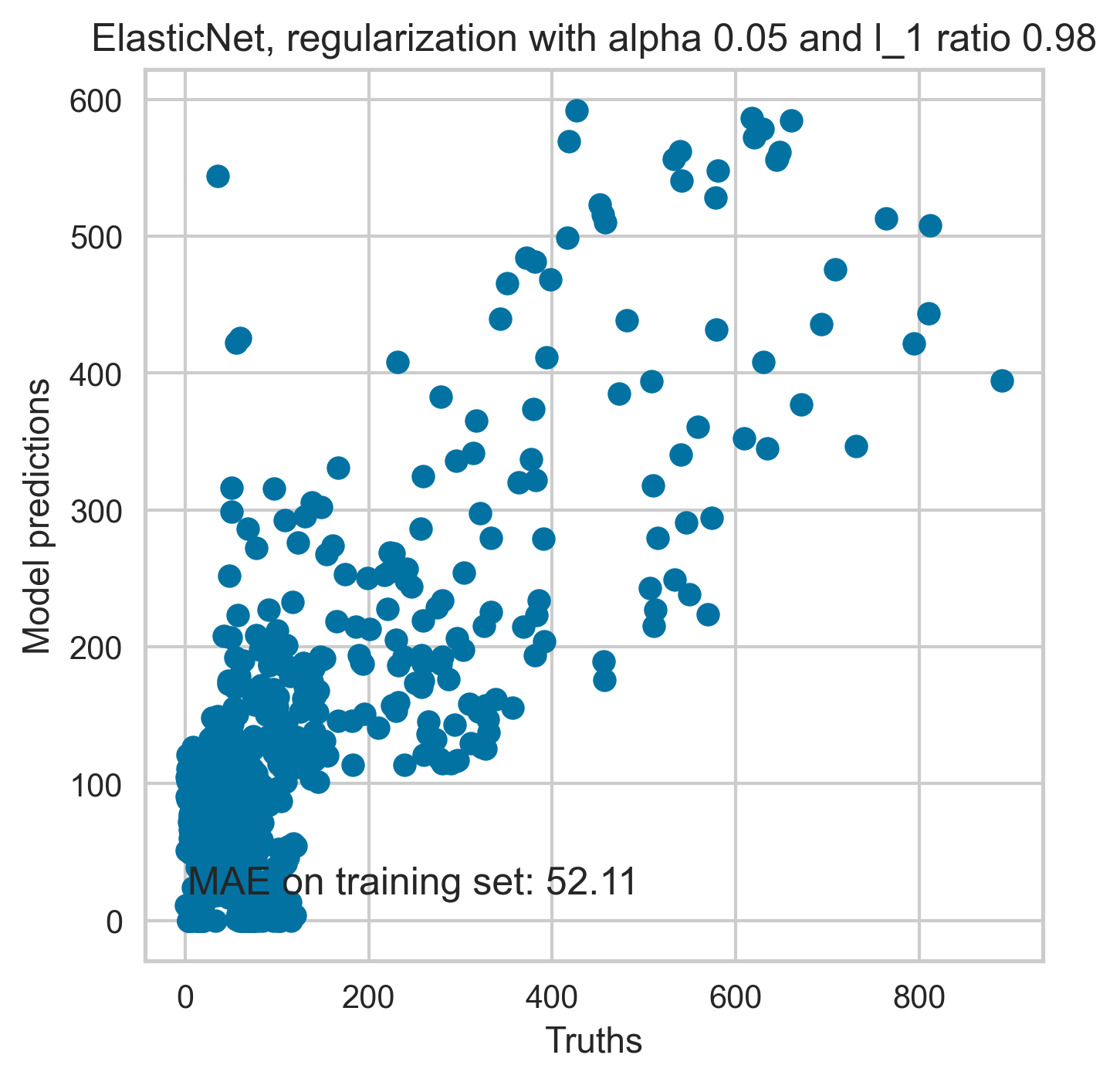
In order to model the influence of multiple predictors on the visitor numbers, we begin with a relatively simple multivariate linear regression model using static and dynamic predictors as the independent variables and the visitor observational count as the target variable.
We tested linear regression with and without regularisation and found that linear regression approach with and without regularisation provided qualitatively similar results. Here we are reporting the analysis from both of the approaches. Including regularisation, although it helps avoid overfitting in forecasting, produces somewhat biased estimation as it adds an extra term to the cost function.
Therefore, we decided to use linear regression without regularisation to report unbiased significant predictors and associated p-values. Linear regression with added regularisation was used to predict visitor numbers on unseen data where unbiased estimates of the coefficients is not of primary interest.
Significant predictors influencing visitor numbers
Table 7 presents the findings from multivariate linear regression based on static and dynamic predictors. Standardised regression coefficients of static and dynamic influences in addition the respective p-values are reported. The reason we have reported standardised regression coefficients is because not all features in our model are measured on the same scale and we need to use the standardised version of their coefficients to compare different features with each other.
In terms of standardised coefficients, a change of one standard deviation in the predictor is associated with a change in the standard deviations of the dependent variable with the magnitude of the corresponding standardised coefficient. As noticed in Table 4, both the dynamic predictors included in our model are statistically significant (pval < 0.05) positive predictors of the visitor numbers in outside natural spaces.
Likewise, areas with higher proportion of population group from Asian/Asian British is a significant positive predictor of the visitor count and so is the proportion of households with two or more cars or vans. Referring to the outputs of the exploratory factor analysis in Table 1 we can get some more insights into some of these predictors.
We can see that areas with higher proportion of population group from Asian/Asian British have high to moderate spatial overlap with areas with higher proportions of bigger households and younger population groups. Moreover, areas with higher proportion of households with access to multiple private cars/vans are less densely populated areas and this is reflected in the observation that visitor count is higher in more rural and less dense urbanised areas (population density is a negative predictor of the observation count).
Other significant positive predictors include camp sites, guest house, bus stops, food court, shelter. Higher densities of these amenities and attractions positively influence the visitor numbers. Density of pubs is the only points of interest feature which has been found to be a negative predictor for time series observational count.
We plan to revisit analysing some of these findings in a future investigation with access to more diverse training data. Lastly, more accessible blue spaces area also results in corresponding upward shift in visitor number in outside spaces. As reported earlier, we experimented with multivariate regression models with and without regularisation to model the visitor numbers in outside spaces and obtained qualitatively similar results.
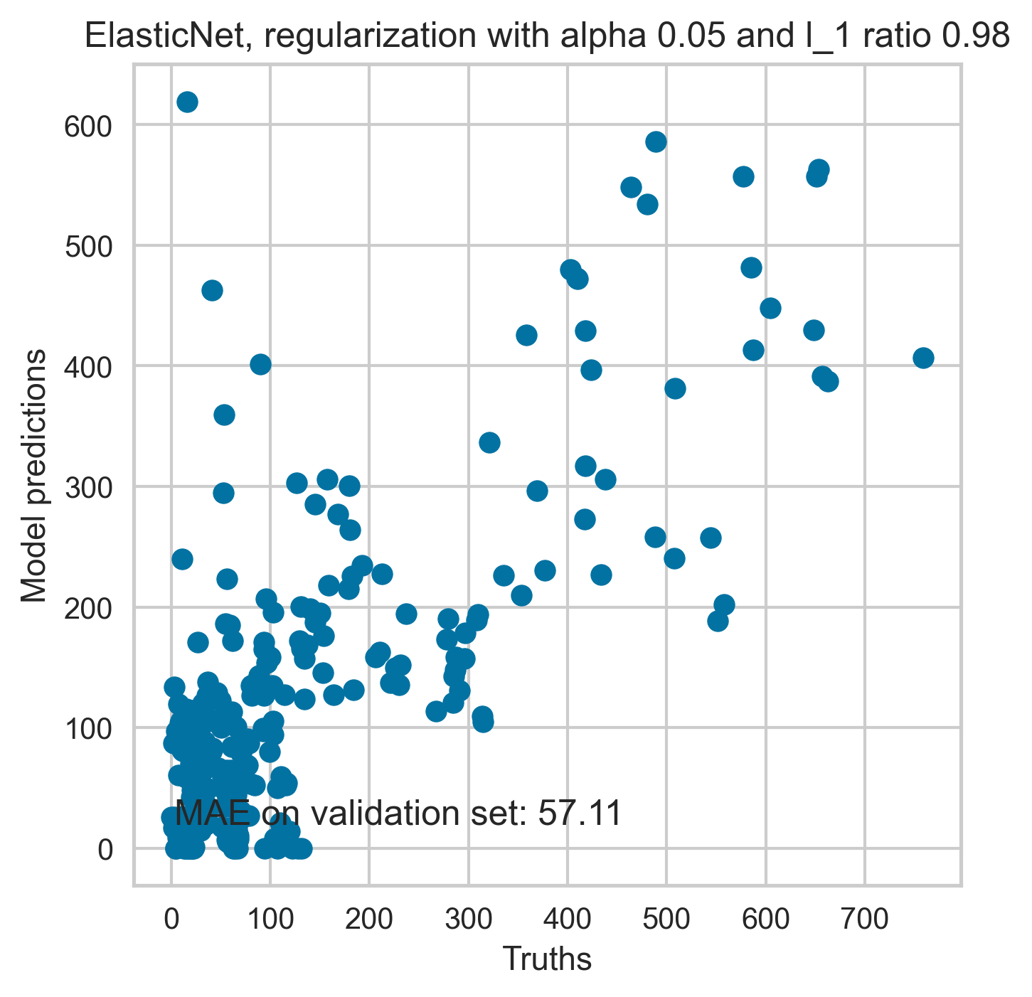
The predictions from a linear regression model with added regularisation is shown in Figure 18. The optimal model parameters used in obtaining predictions reported in Figure 18 are obtained following tuning of hyperparameters (alpha and l1).
Table 7. Standardised static and dynamic predictors influencing visitor count in selected natural spaces in England covering the period January 2020 to November 2022.
| names | coef | se | T | pval | r2 | adj_r2 | CI[2.5%] | CI[97.5%] | ||
| Mean dog occupancy | 0.04 | 0.03 | 1.24 | 0.21 | 0.68 | 0.67 | -0.02 | 0.10 | ||
| waterside length km | 0.24 | 0.04 | 6.81 | 0.00 | 0.68 | 0.67 | 0.17 | 0.31 | ||
| land type labels urban and rural settings | 0.17 | 0.05 | 3.64 | 0.00 | 0.68 | 0.67 | 0.08 | 0.26 | ||
| habitat type labels Grass wood bareground coast | 0.03 | 0.03 | 0.89 | 0.38 | 0.68 | 0.67 | -0.03 | 0.09 | ||
| tourism camp site | 0.24 | 0.03 | 7.51 | 0.00 | 0.68 | 0.67 | 0.17 | 0.30 | ||
| tourism guest house | 0.41 | 0.04 | 10.62 | 0.00 | 0.68 | 0.67 | 0.33 | 0.48 | ||
| highway bus stop | 0.33 | 0.05 | 6.15 | 0.00 | 0.68 | 0.67 | 0.22 | 0.43 | ||
| tourism attraction | -0.01 | 0.03 | -0.46 | 0.64 | 0.68 | 0.67 | -0.07 | 0.04 | ||
| amenity pub | -0.34 | 0.04 | -7.95 | 0.00 | 0.68 | 0.67 | -0.43 | -0.26 | ||
| amenity beer garden | -0.00 | 0.04 | -0.06 | 0.95 | 0.68 | 0.67 | -0.07 | 0.07 | ||
| amenity bus station | 0.03 | 0.04 | 0.70 | 0.48 | 0.68 | 0.67 | -0.05 | 0.10 | ||
| amenity food court | 0.22 | 0.03 | 6.90 | 0.00 | 0.68 | 0.67 | 0.16 | 0.28 | ||
| amenity shelter | 0.11 | 0.03 | 3.40 | 0.00 | 0.68 | 0.67 | 0.05 | 0.17 | ||
| Asian/Asian British | 0.41 | 0.06 | 7.46 | 0.00 | 0.68 | 0.67 | 0.30 | 0.52 | ||
| 2 or more cars or vans in household | 0.23 | 0.07 | 3.45 | 0.00 | 0.68 | 0.67 | 0.10 | 0.36 | ||
| Density (number of persons per sq km) | -0.25 | 0.05 | -4.65 | 0.00 | 0.68 | 0.67 | -0.35 | -0.14 | ||
| total trip count | 0.33 | 0.03 | 11.68 | 0.00 | 0.68 | 0.67 | 0.28 | 0.39 | ||
| tavg | 0.12 | 0.02 | 4.98 | 0.00 | 0.68 | 0.67 | 0.07 | 0.17 | ||
Figure 18. Prediction of the model on the train dataset (Top) and held out validation set (Bottom).
Variability of predictors
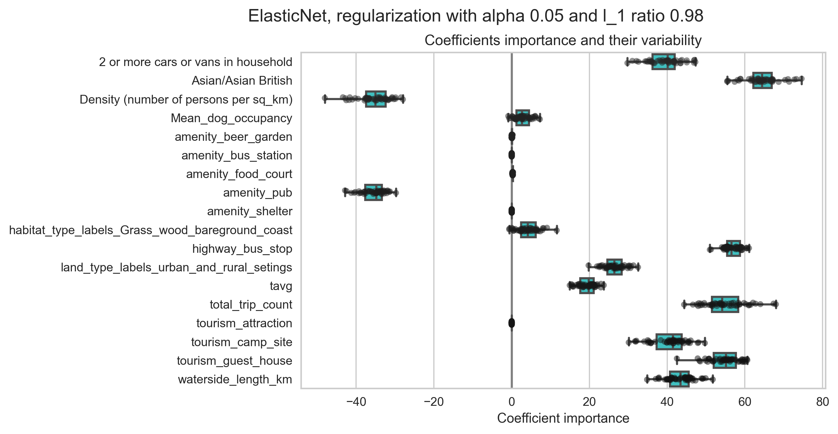
This section evaluates the extent to which the identified static and dynamic predictors have been stable over time. We can check the coefficient variability through repeat k−fold cross-validation which is a form of data perturbation. k−fold divides the data into k non-overlapping parts (called folds), hold out one of these folds and use the remaining folds (k−1) to train a model.
This process is repeated across all the folds until all the data has been used. To reduce potential biases, one can also repeat the k−fold cross-validation procedure multiple times and report the results across all folds from all runs. Figure 19 reports the regression coefficients of a regression estimator with regularisation obtained for all folds from all runs.
The model with regularisation is the same as used for obtaining the predictions presented in Figure 18. If estimated coefficients vary significantly when changing the input dataset their robustness is not guaranteed and they should probably be interpreted with caution. The results reported in Figure 19 are qualitatively similar to the standardised linear regression coefficients reported in Table 7.
It can be verified from Figure 19 that the predictors with average of their distribution close to zero are not significant as also reported in Table 7. On the other hand, value of the mean of the distribution of a given predictor directs the relationship between the respective predictor and the outcome variable.
Figure 19. Static and dynamic risk predictors variability following a repeated k−fold cross-validation procedure as outlined in the main text. The estimator is a linear regression with added regularisation with optimal parameters obtained after tuning of hyperparameters as described in the main text.
Visitor estimation for spatial locations
One of the main advantages of a machine learning model is an adequately trained model can learn from the past and is capable of making predictions for the future. Ideally, a good machine learning based model should be able to make sufficiently accurate and data-driven decisions.
With this motivation, in this section we will present the predictions obtained from a trained estimator with a view to providing a spatially and temporally granular estimate of the numbers of visitors visiting outside natural spaces.
Prediction on spatial sites in the training dataset
As a first step to assess the performance of our trained estimator, we hold out part of the available data and call it a test dataset and the rest of the data are used for training an estimator. The optimal model is selected using a cross validation process and grid search. The entire model training workflow is shown in Figure 20.
In the anticipation of future access to a more diverse training data, we make use of an automated machine learning workflow to develop an ensemble estimator which combine the predictions of several base estimators to improve generalisability/robustness over a single estimator.
The focus of this section is on choosing the most suitable estimator which once trained can be used to estimate visitor counts in new spatial locations for different time periods. We thus do not constrain ourselves to model the relationship between the predictors and the outcome variable using a linear regression model but explore a range of linear and non-linear regressors.
There are various ways to combine different base estimators to create an ensemble estimator. In the previous sections, we have experimented with linear regression with and without added regularisation to estimate observational count time series data.
Instead of using these estimators separately, in this section we focus on combining these different estimators to build an ensemble estimator. We have experimented with two different ensemble regressors: Voting regressor and Stacking regressor.
A voting regressor is an ensemble meta-estimator that fits several base regressors, each on the whole dataset. Then it averages the individual predictions to form a final prediction. A stacking regressor is a stack of estimators with a final regressor and it allows to use the strength of each individual estimator by using their output as input of a final estimator. A visual representation of the two ensemble regressors is shown in Figure 21.
We compared the performance of the two ensemble regressors using a cross validation workflow the model performance metrics are shown in Table 9 and 10. The voting model slightly outperforms the stacking model and therefore the voting ensemble regressor was chosen as the final model and used for all future predictions. Figure 22 shows the predictions from the voting ensemble regressor compared against ground truth people counter data for each region in England.
Figure 20. A cross validation workflow in model training.
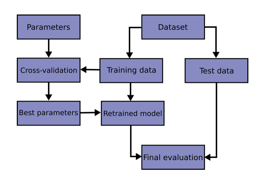
Figure 21. Two ensemble regressors investigated: Voting regressor and Stacking regressor

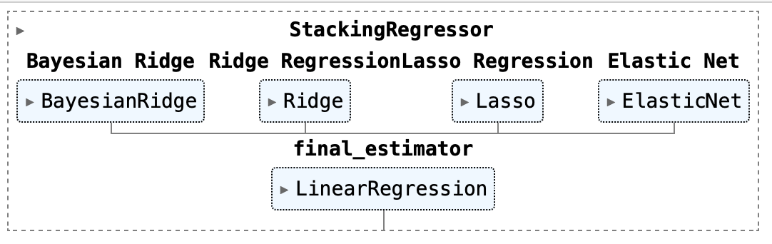
Table 8. Model performance metrics for voting ensemble model
| Fold | MAE | MSE | RMSE | R2 | RMSLE | MAPE |
| 0 | 65.86 | 8236.92 | 90.76 | 0.68 | 0.97 | 1.93 |
| 1 | 82.71 | 15994.24 | 126.47 | 0.52 | 1.26 | 3.09 |
| 2 | 77.25 | 16564.34 | 128.70 | -0.15 | 1.16 | 2.89 |
| 3 | 94.74 | 16664.09 | 129.09 | 0.63 | 1.08 | 2.24 |
| 4 | 74.83 | 10890.41 | 104.36 | 0.62 | 1.02 | 1.67 |
| Mean | 79.08 | 13670.00 | 115.88 | 0.46 | 1.10 | 2.36 |
| Std | 9.54 | 3463.77 | 15.59 | 0.31 | 0.10 | 0.55 |
Table 9. Model performance metrics for stacking ensemble model
| Fold | MAE | MSE | RMSE | R2 | RMSLE | MAPE |
| 0 | 62.98 | 7068.91 | 84.08 | 0.72 | 1.01 | 2.00 |
| 1 | 76.33 | 13095.32 | 114.43 | 0.60 | 1.19 | 3.07 |
| 2 | 70.32 | 13445.81 | 115.96 | 0.07 | 1.11 | 2.65 |
| 3 | 88.10 | 14811.94 | 121.70 | 0.67 | 1.03 | 2.28 |
| 4 | 69.53 | 8653.30 | 93.02 | 0.69 | 0.96 | 1.58 |
| Mean | 73.45 | 11415.06 | 105.84 | 0.55 | 1.06 | 2.32 |
| Std | 8.46 | 3000.08 | 14.60 | 0.24 | 0.08 | 0.52 |
Figure 22 (a) Comparison of Actual People Count and Predicted People Count time series for each region in the England using voting ensemble model. (b) Comparison of RMSE for Voting Ensemble model and base linear regression model for each region of Egland. Please refer to Figure 26 for the number of sites in training data for each region.
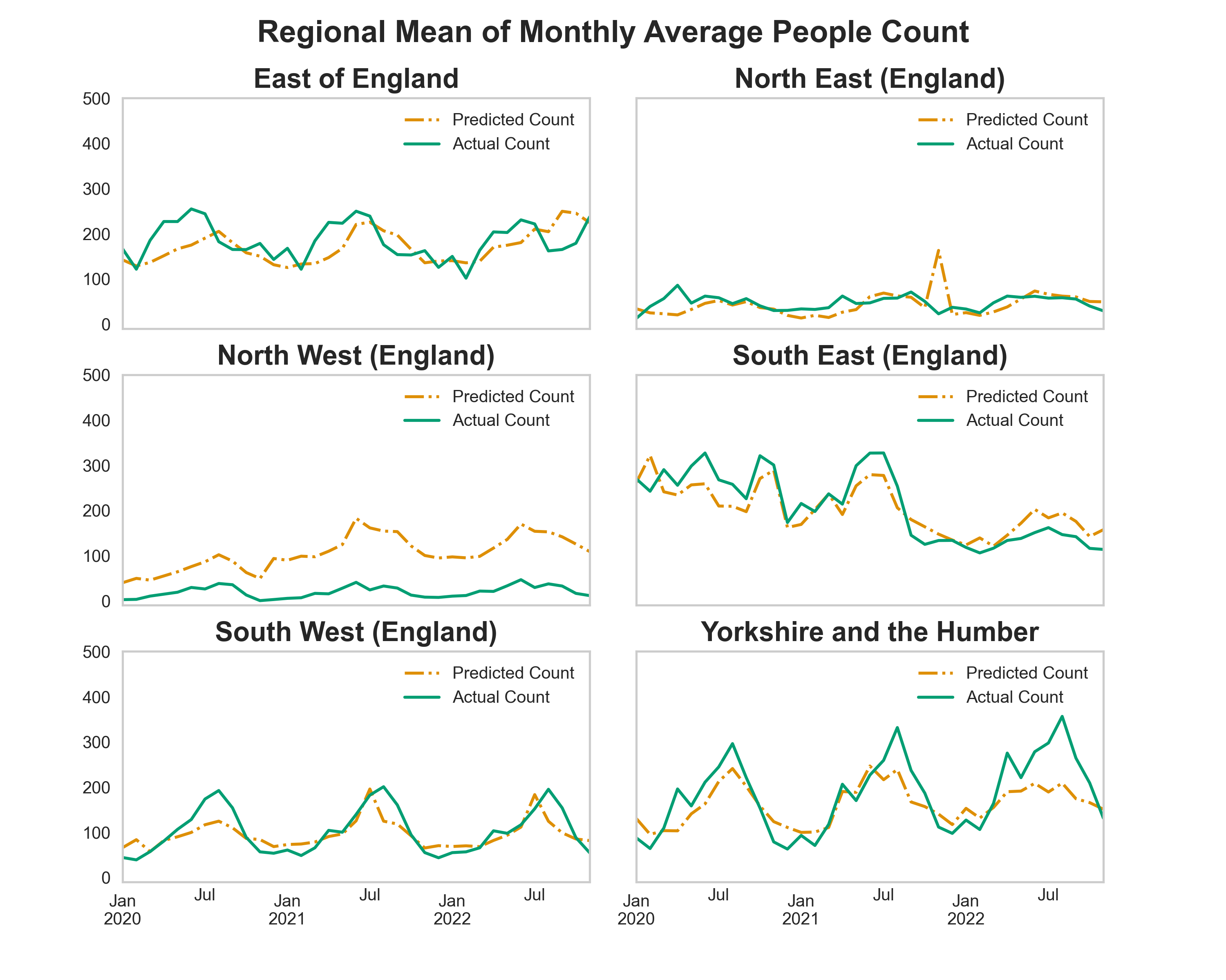
Figure 22 A
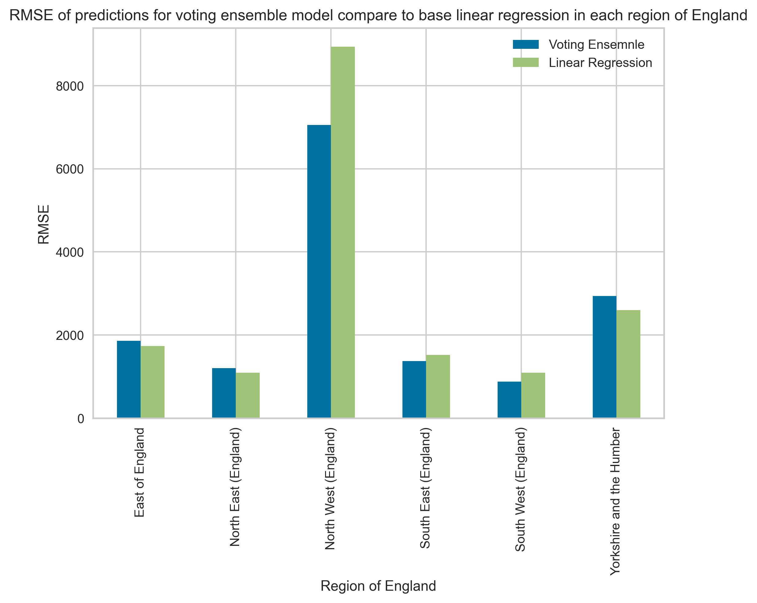
Figure 22 b
Figure 23. Map of People Counter Sites coloured by region and table of number of people counter sites per region
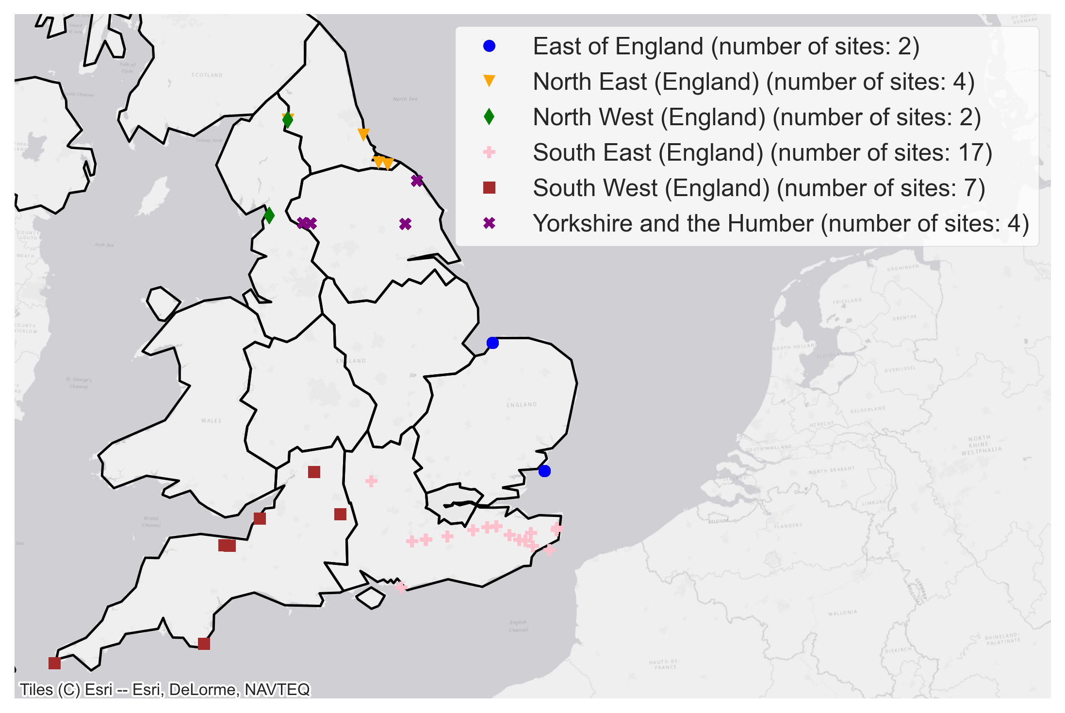
Figure 22 shows the performance of the model when making predictions on train and test data sets compared with the ground truth people count numbers. When comparing Figure 22 with Figure 23 it is clear that the model performance is better for regions that have a larger number of corresponding sites.
For example, model predictions in South East and South West regions are more similar to the Actual Count than the predictions in North West and North East regions. Across South East, South West and Yorkshire and the Humber regions the model predictions successfully capture annual seasonal trends present in the Actual Count data. Excluding predictions made in the North West region the absolute value of predicted count made by the model are similar to the absolute values in actual count data.
Prediction on spatial sites outside the training dataset
In the previous sections, we tested the performance of trained estimators on separately held (unseen) training data. This provides us with a useful metric to assess the performance of our model. Another possibility that could be of interest is to use a trained estimator to estimate visitor count for spatial sites not included in on the ground people visitation time series training data.
This can be a useful output from our approach as it will allow us to generalise the estimates from our model to a much wider spatial area and contribute towards developing more representative regional estimates of visitors to natural spaces.
We follow the following steps to identify sites which are not part of the observational count time series data but for which visitor count can still be potentially estimated using our trained estimator:
- We fix the estimator to be an ensemble regressor trained using a cross validation workflow as outlined in the previous section.
- The people monitoring sites operated by the potential data provider form our pool of sites for which we want to estimate the visitor numbers. Do note that we do not have access to the observational count time series data for these additional sites. However, we have made use of the locations of these additional sites to prepare the static and dynamic predictors used for training the ensemble regressor.
- For a fixed site amongst these additional sites, we find its nearest neighbour from the sites in the training dataset. The nearest neighbour is found based on the minimum distance between the two vectors and uses a tree based algorithm. Each component of the vector represents one of the static features for each corresponding site. This process is then repeated for all other additional sites.
- Neighbour of each additional site in the training data are reported along with the nearest neighbouring distance. Only those additional sites with the nearest neighbouring distance falling in the first quartile (Q1) are considered valid for visitor count estimation. These are the sites which are expected to be most similar to the sites present in the training data and our trained estimator is expected to perform well in estimating visitor counts for these spatial locations. This hypothesis is to be tested once we have access to ground truth people visitation time series data for these additional sites.
- A frequency count of the additional sites and their neighbouring training sites is observed to identify most similar training sites. The top-10 sites in the training dataset with the highest number of neighbouring sites amongst the additional sites are chosen as the representative sites in the training dataset as shown in Figure 24. This cut-off is somewhat arbitrary we should stress.
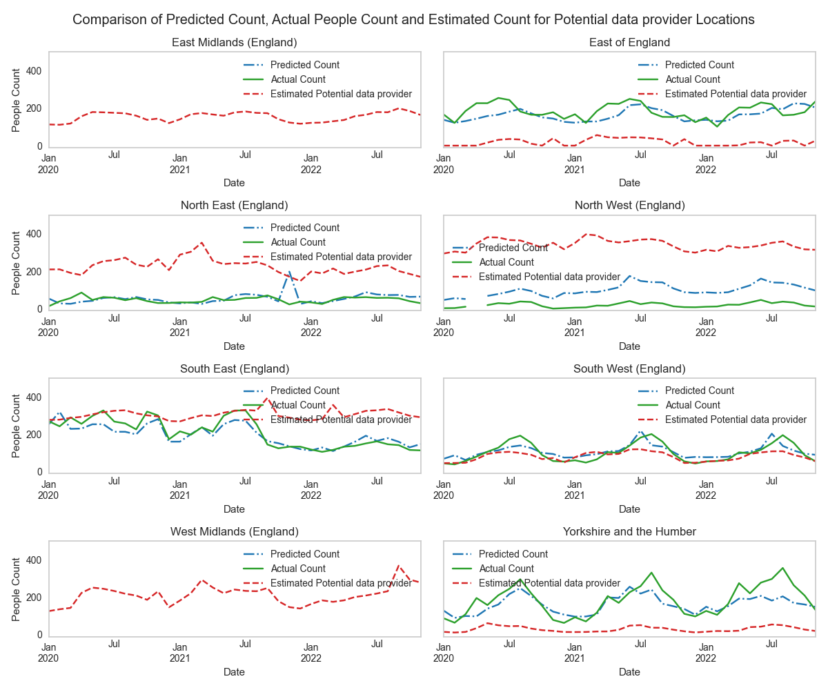
- Finally, the trained estimator is used to make estimations for visitor count for these chosen additional sites. Figure 25 shows the predictions from the trained estimator on a sample of the sites from the potential data provider network which have been deemed most similar to some of the sites present in the training data. The values shown are the mean people count numbers for all sites in each region.
Figure 24. Shown here are the sites in the training data and their identified neighbours in the potential data provider monitoring network. It is worth noting that spatial proximity alone does not guarantee that any two given sites will be identified as neighbours.
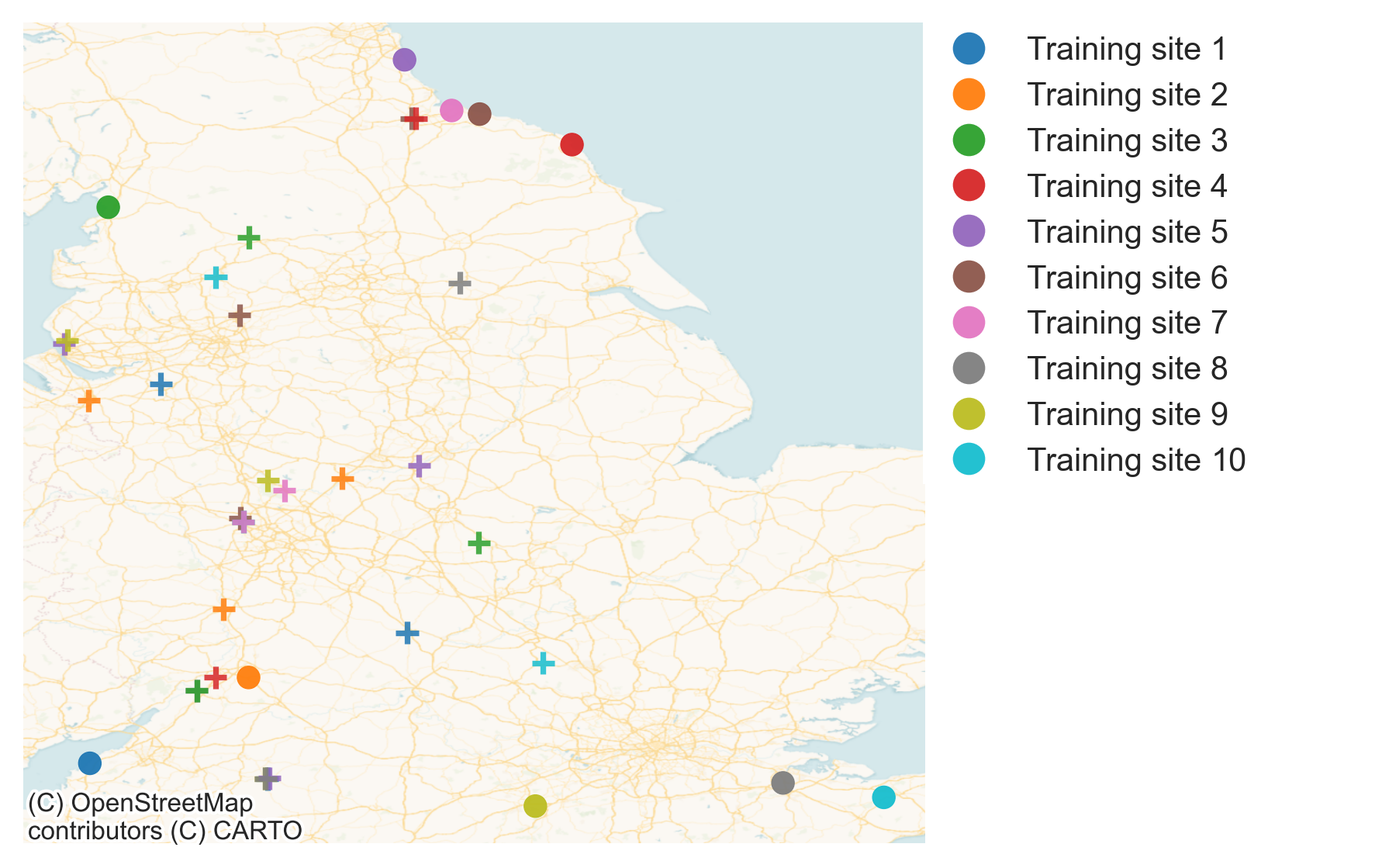
Figure 25. Comparison of Actual People Count, Predicted People Count and Estimated people count for Potential data provider sites
7. Conclusions and limitations
In this experimental investigation, aggregated anonymised Strava pedestrian activity data alongside carefully selected static and dynamic features have been shown to model visitor numbers in chosen spatial locations.
A fully reproducible machine learning pipeline has been built to model observational time series count based on non-disclosive open data sources. Machine learning pipeline has been used to predict visitor count on held out test data and unseen new spatial location.
As has been found in related investigations exploring other big data sources for estimating visitor numbers in outside natural spaces, Strava Metro data too it seems will require correction (re-scaling) to match the scale of on the ground observations and more good quality and diverse on ground observation training data are required to develop this recalibration scale.
We have attempted to model on the ground people counts time series using a series of modelling approaches, including panel data structure and fixed effects approach and multivariate regression analysis. Both these approaches result in our finding that there exists statistically significant positive relationship between the pedestrian Strava activity count, chosen spatial features and on the ground observational time series.
As is true for most modelling approaches, ours too has its limitations. Firstly, a lack of more diverse training data are a big limitation in extrapolating our findings to produce regional or national estimates of visitors visiting outside natural spaces.
Estimates of visitors for selected spatial locations are point estimates. More work is required to convert these (raw) predictions to area adjusted visitor footfall in selected areas. Road disruption and traffic congestion is expected to play a key role in affecting the visitors count in selected locations.
Model outputs can certainly benefit from incorporating this information along with accessibility information such as frequency of trains/buses for example for the chosen spatial sites. Analysis can further benefit from updating the socioeconomic and demographic features with the Census 2021 information. At the time of writing this report, Census 2021 does not provide all features at the required spatial granularity used in the modelling.