Supporting healthcare guidance recommendations using natural language processing

The Data Science Campus ‘Enable’ programme is aimed at strengthening data science capability across the public sector, and you can read about more of our work on the data science accelerator, graduate programme and much more in our capability pages. This work includes supporting public sector organisations to use data science tools and techniques in their daily operations, to go faster, improve quality, and reduce costs.
This article describes our work with the National Institute for Health and Care Excellence (NICE) to identify documents and recommendations that are relevant to guidance that is under review by NICE. The project was carried out in three major parts:
- data-engineering, where the existing recommendations and guidance data were web-scraped from NICE’s application programming interface (API) and put into a structured JSON data format
- natural language processing (NLP) exploratory research, which evaluated several models and data augmentation methods
- putting project deliverables into a production environment on NICE servers for live use
The project was successful in delivering significant and proven improvements to NICE’s surveillance operations in both accuracy and processing time.
This report describes the technical work and design choices made during the exploratory and delivery phases of the work.
1. Introduction
The National Institute for Health and Care Excellence (NICE) provide national guidance and advice to improve health and social care practices, organised as guidance products. These guidance products were stored in HTML format with no clear distinction between the text sections within guidelines. The data records described must be kept up to date with state-of-the-art healthcare practices, which evolve daily through new research. Our research project used state-of-the-art natural language processing (NLP) practices to help NICE build a mechanism to query related recommendations throughout their dataset given an input recommendation.
Motivation
In NICE, the surveillance team is responsible for assessing whether any new evidence impacts on the existing guideline recommendations. With over 300 guidelines, each containing hundreds of recommendations as well as other textual information, this is no small task. One key element of the guideline review process is the identification of overlapping content. NICE needs to make sure that it is consistent in its recommendations and there are no contradictions between guidelines. Checking related guidelines is a manual, time-consuming task as content is stored on the website. For any given guideline, up to a week of an analyst’s time may have been spent checking other guidelines for overlaps. This task was challenging primarily because NICE did not have a searchable structured database of its recommendations for a keyword search.
Figure 1: A screenshot of NICE’s website showing a guidance page.
The rest of this report is structured into three categories, including:
- data: a section describing the data and the data-engineering phase of the project
- methods: a section describing the NLP models evaluated in this project as well as the benchmarking mechanism employed to rank them
- results and discussion: a section listing our best results as well as comments
2. Data description for the National Institute for Health and Care Excellence
When developing a guideline, the National Institute for Health and Care Excellence (NICE) uses Microsoft Word files as the main publishing software for guideline documents. A guideline can amount to thousands of pages when including all the methods, analysis and interpretation of the evidence leading to the recommendations. These long and complex documents are generally converted to PDF format and hosted on the guideline webpages (see Figure 1 for an example). The recommendations and other key information are converted directly from a Word file to HTML for display on the NICE website.
When searching for existing recommendations, NICE staff used the NICE website to search for relevant guidelines or recommendations. Although a keyword search within the NICE website was available, this returned webpages rather than specific recommendations. Analysts needed to read through or use a “browser find” function to search to find the specific recommendations of interest. They also needed to manually record their findings.
This method was inefficient in many ways. An analyst needed to read potentially thousands of recommendations to find a few relevant recommendation relationships. The number of recommendations per guidance product ranges from 417 to 4,891 at the time of publication, with 17 out of 19 topics consisting of more than 1,000 recommendations. A breakdown of the guidance products per topic is presented in Figure 2. The website keyword searching would not capture all synonyms or changes in terminology over time, so results could be incomplete. Similarly, the searches would be influenced by an individual’s pre-existing knowledge of the topic area, so results could be expected to differ depending on who did the searches. Finally, decisions about which recommendations were considered to be related could differ between individuals and so were not entirely objective, and the recording of findings was subject to human error.
Figure 2: Number and percentage of recommendations in NICE guidelines, by theme of the guideline. NICE guidance products, such as technology appraisals, are not included in this list.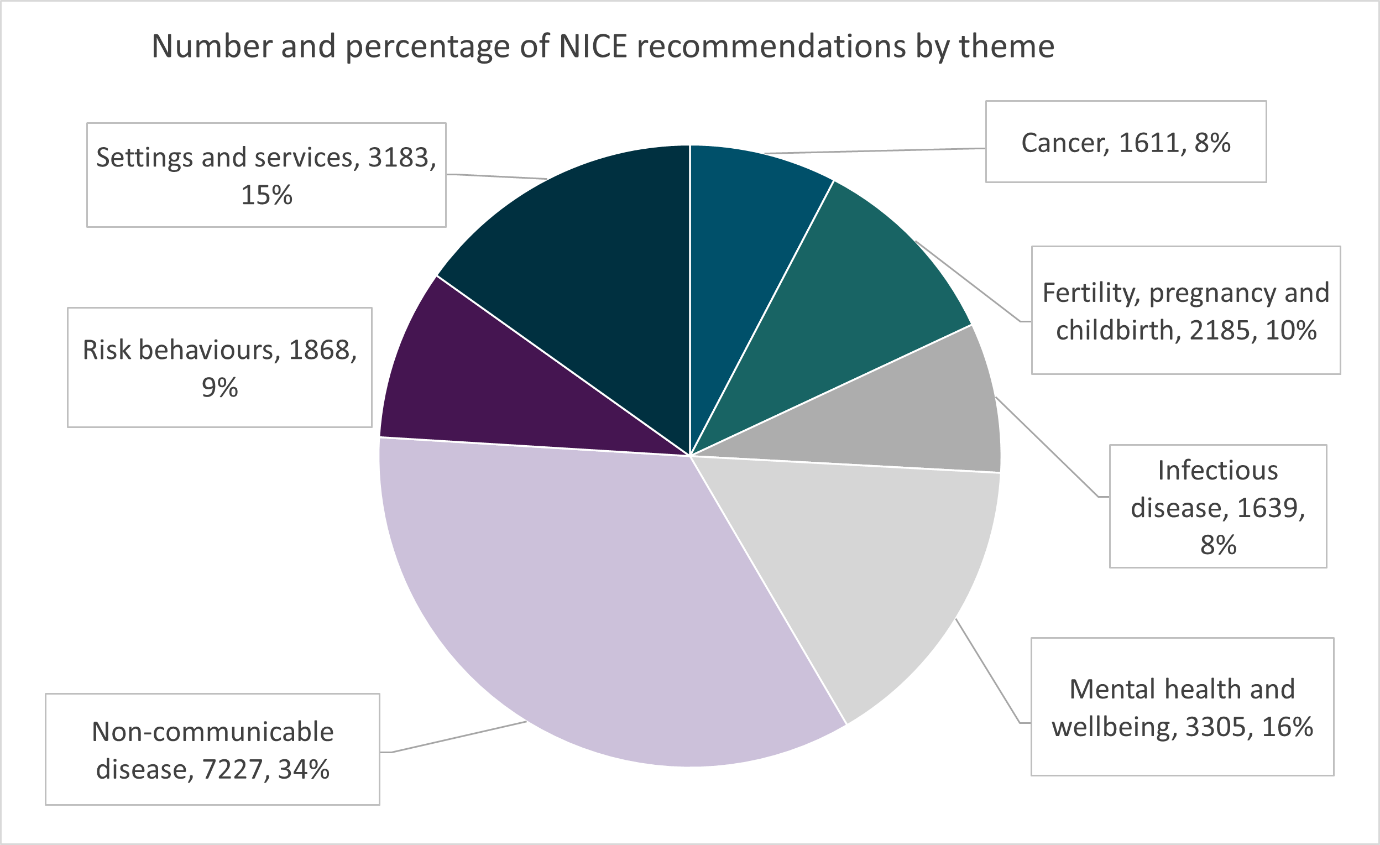
3. Data engineering
To perform any cutting-edge natural language processing (NLP) methods, we needed to apply structure to the data, because we only needed the recommendation text out of each guideline. Unfortunately, the recommendation text inside guidelines was not structured in a consistent way. We (Data Science Campus at the Office of National Statistics)worked with the National Institute for Health and Care Excellence (NICE) to find patterns for certain guideline groups so that we could extract most of the recommendations using web scraping, creating a state machine to map text to structure.
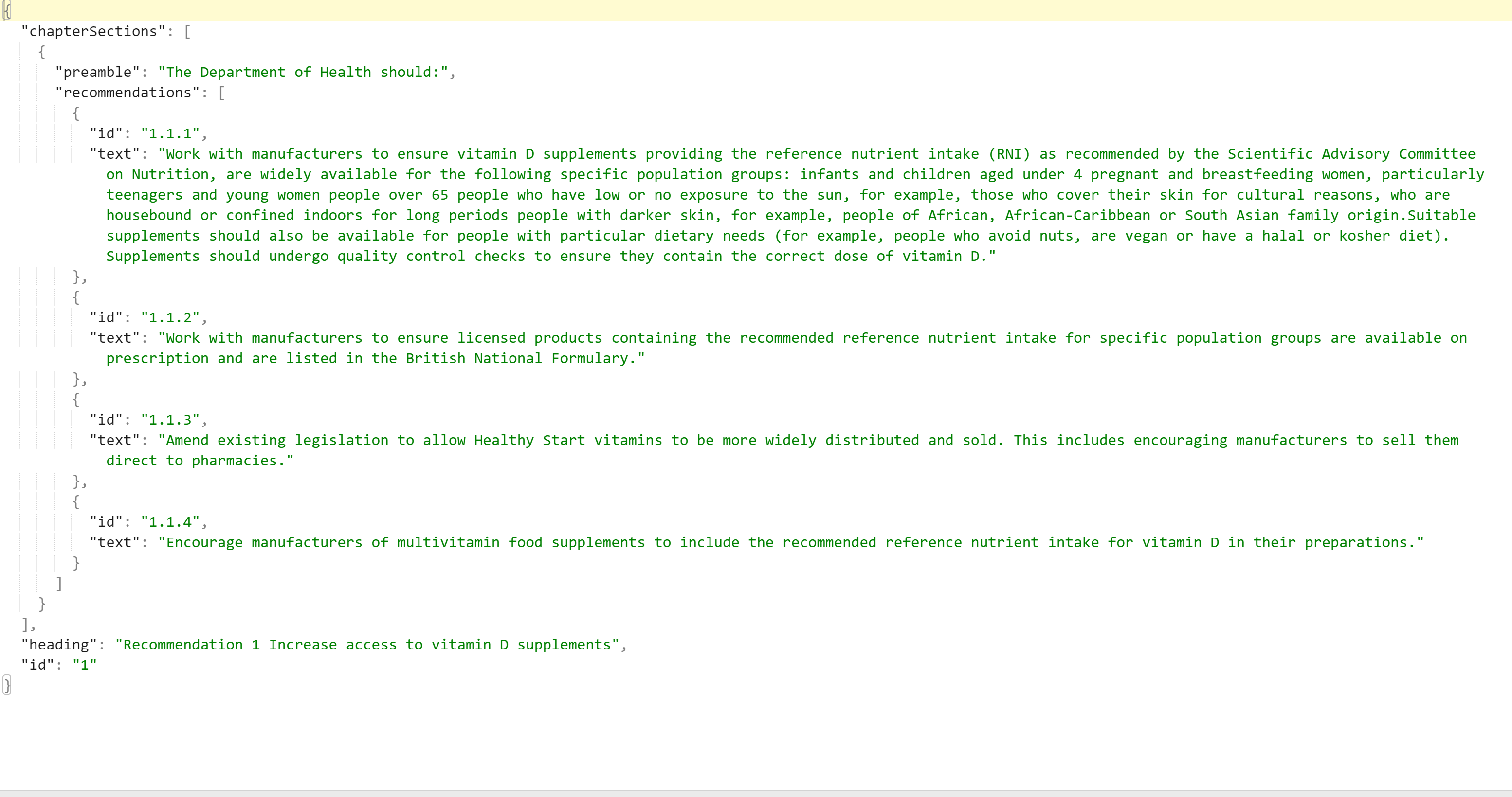
During this process, we aimed to give a unique index (ID) to each section inside a guideline, creating a hierarchical JSON structure, as depicted in Figure 3. Every guideline listed recommendations, and every recommendation listed sections, and every section listed of paragraphs and/or sections, and every paragraph contained the underlying text. This underlying text we now refer to as the actual recommendation.
Note that the depth of the hierarchy varies depending on the structure of the individual guideline – some had sections and some had sub-sub-sections, all with slightly different formatting. These recommendations were then given a unique ID, so that our matching algorithm could return their IDs, rather than their text. Out of this JSON file, we extracted only the recommendations for our modelling work, and each recommendation had a composite key, namely <guideline ID, paragraph ID>. We need to mention here that the paragraph ID consisted of three parts, which are the recommendation ID, the section ID and the paragraph ID, as depicted in Figure 3.
We performed quantitative and qualitative tests to measure the success of this operation, and both estimated it to be over 95%. The test criteria were the number of guidance products and recommendations successfully web-scraped and appended into our structured dataset compared to the total number of guidance products and recommendations that were estimated by NICE. A reporting mechanism was applied to our web-scraping data-engineering process to report when there were issues with the process, such as text that could not be extracted and missing paragraphs, for example. Manual random sampling was also used to ascertain the accuracy of the process, as explained in the Data Testing section. The outcome of this random sampling was taken into consideration when applying the necessary changes to the web-scraping code to further improve the completeness of the resulting structured dataset.
Figure 3: Example dataset structure on completion of our data engineering phase.
| JSON element | Types of content | Examples |
| Guidance product | Title
Heading ID List of Chapters of Recommendations |
Fractures (non-complex): assessment…
NG38 |
| Chapters of Recommendations | Heading
ID Preamble List of Chapter Sections |
Initial pain management
1 ‘preamble text prior to each chapter section’ [optional] |
| Chapter Section | Heading
ID Preamble
List of Recommendations List of Chapter Subsections |
Pain assessment
1.2 ‘preamble text prior to each chapter subsection’ [optional]
[optional] |
| Chapter Subsection | Heading
List of Recommendations List of Chapter Subsubsections |
Pain assessment
[optional] |
| Chapter Subsubsection | Heading
List of Recommendations |
Pain assessment |
| Recommendation | ID
Text |
1.2.1 or 1.1.1.3
We recommend that… |
Figure 4: A snapshot from our resulting JSON file.
4. Data testing
Testing by inspection was conducted to ensure the data extraction was accurate. This testing involved comparing the recommendation content extracted using the data-engineering approach described above with the guideline content on the National Institute for Health and Care Excellence (NICE) website. A random sample of 10% of all recommendations (n=2,077) were inspected manually by domain experts. On evaluating the errors, only 70 error reports were classed as true errors and generally fit into four broad categories. A major issue identified at this stage was that older public health guidelines had a different structure, which meant that extra code was needed to split and number individual recommendations. The remaining three broad categories of errors identified were headings missed because of a non-standard structure in the source guidance, non-recommendation paragraph text being included, and table content identified inconsistently.
The feedback from this manual inspection was used to apply any necessary changes to the data-engineering approach. Because the error rate was so low in the first analysis, no further systematic validation of the data-engineering output was needed.
5. Methods
Verification and validation plan
Once the data-engineering work was complete, we were faced with a plethora of algorithms and models that could help with this task, including:
- CountVectors (TFIDF)
- Word2vec
- fastText
- bioword2vec
- ELMO
- BERT
- BioBERT
- XLNet
- and others
The question at this point was: which one? There were several publications comparing the above, however each corpus and task can be different. We decided to create a verification and validation (V&V) framework to assess several models that we considered fit for this task. The process of creating this V&V file for each of the two recommendation link tasks included the following steps:
- we asked the National Institute for Health and Care Excellence (NICE) to provide a set of surveillance queries (<=100) using their existing methods; we will refer to this as phase 1 of the process
- each query would have their associated recommendation results and we would use this file as a standard (we will refer to it as the “NICE Standard” set) to assess several algorithms and models
- next, we used our models to score all the recommendations in our dataset, once for each query against the NICE standard set; then, for each query, we ranked the results from the highest to the lowest score
- we then scored the models by the number of (known) true positives that they were able to recover on their top-200 recommendation links for each query, and then picked the outputs from our best model and sent the results back to domain experts; he known true positives were annotated with a flag (1) to indicate that they belonged to the NICE standard
- the domain experts would, in turn, annotate the newly retrieved true positives with the label ‘2’; we called this phase 2 of the process, and these would be true positives that were recovered by the model, but not from experts on their initial evaluation
- the union between the new set of labels and the old ones from the NICE standard would become our new “Gold Standard”; this new set would be the basis for further algorithm evaluations, and these new true positives would have been missed by the existing manual process
Verification and validation implementation
This section explains how the verification and validation (V&V) sample was constructed, including phase 1 (National Institute for Health and Care Excellence (NICE) Standard) and phase 2 (Gold Standard).
Phase 1
A convenience sample of surveillance queries was selected to provide data for model testing. Data were collated to test two user cases, which were keyword searching and recommendation searching.
Surveillance subject-matter experts were allocated guidelines and asked to randomly select keywords and recommendations related to their allocated guidelines. To ensure broad coverage of topic areas, one person was responsible for allocations and distributed guideline products across the team. They ensured that all guidance products were in the sample – namely, clinical and public health guidelines, technology appraisals, diagnostic guidance and interventional procedure guidance.
For keyword searches, the relevant term was searched on the NICE website and relevant recommendations, including that keyword, were identified. Data including keyword and output recommendations was recorded in a spreadsheet. For recommendation relationships, the full input recommendation, or keywords from the recommendation, was searched on the NICE website. All data were quality assured by two independent domain experts responsible for surveillance. This dataset was then used by as a basis to evaluate several models.
Phase 2
Model data provided by the Office for National Statistics (ONS) were validated by domain experts responsible for surveillance. Recommendation relationships identified by the model were provided to the National Institute for Health and Care Excellence (NICE) in a spreadsheet. Using pre-specified criteria, relationships between input and output recommendations identified by the model were manually determined as a real relationship or not and decisions were recorded. All manual decisions were independently verified by a second reviewer and any disagreements discussed to reach a consensus. Manual data were fed back to the Data Science Campus to further adjust the model rankings and explore further possibilities. The newly retrieved data by the model were given a label 2 to record that they were recovered by the model but not from NICE in phase 1. The verification and validation workflow is shown in Figure 5.
Figure 5: The verification and validation workflow.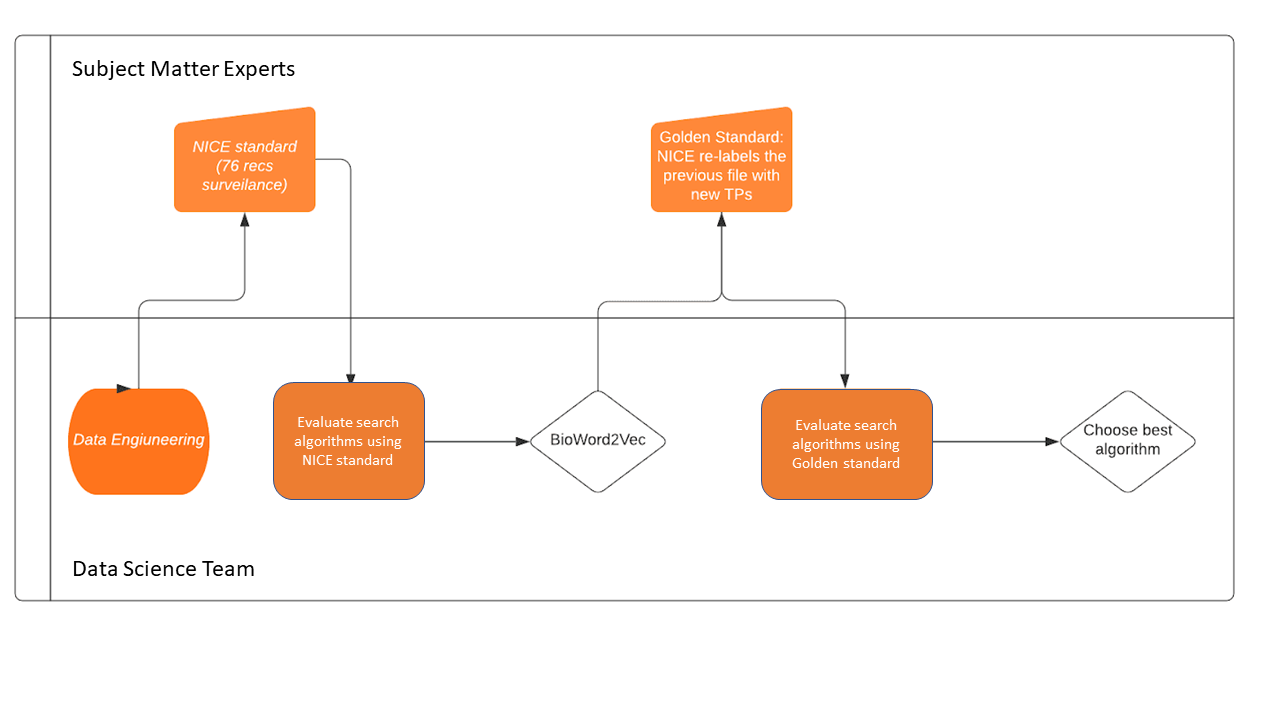 Methods employed
Data augmentation
After the data engineering phase of the project, we inspected the data prior to making decisions on the search algorithms. It quickly became apparent that there were two main issues. The first issue was that some recommendations were extremely short and relied upon context from neighbouring recommendations. The second issue was that some recommendations did not mention the subject matter; this was assumed from the heading.
We investigated these issues and came up with solutions described in the following sections.
Load balancing
We attempted to resolve this issue by grouping small recommendations (whose word count fell below a certain threshold) that belong to the same parent section. This way we could ensure that contextless recommendations would inherit context from a richer paragraph in word count and appear in search results. We used this method to compare against non-load-balanced datasets and then pick the best performing one. Different levels of load balancing were tried, with thresholds of [50, 100, 150] word counts and with groupings on section level and on recommendation level.
The grouping was done using a greedy algorithm approach. This means that, for every given level, (such as chapter-of-recommendations, chapter-of-sections and recommendations), we sorted the recommendations text by word length. Then starting from the top recommendation (pivot point – highest word count), we would construct and probe groupings of recommendations below it (including self) and keep the grouping closest to the given threshold. The groupings would be assessed with the score of the pivot recommendation on its own, too. This is because, in some cases, such as group on recommendation level with threshold 50, most recommendations would not require grouping. Once the top scoring grouping was found, the constituent recommendations were removed from the pool and merged into the processed data frame, along with the necessary information to decompose at a later stage.
Additional context information
An alternative method of adding context to the recommendations was by prefixing each recommendation with the guidance product title, and any headings or preambles that logically precede each recommendation within the hierarchy structure of the guidance product.
Figure 6 shows the word length distributions of load balancing on different section levels and different thresholds. The reason why the datasets suffixed with “lemma” have a smaller variance compared to their non-lemmatized equivalents is because these datasets have kept nouns only from each sentence, hence the lesser word-count. The dataset preceded by ‘_cn’ is the one augmented with header and pre-amble information. This plot helps understanding of the impact of load balancing on the data by looking at the shift of the wordcount distributions compared to plain recommendations, as shown on the first boxplot on the graph. For example, if we look at the chaptersOfRecommendations-level data (one before last) along with its load-balanced sets (lb_50_ chaptersOfRecommendations and lb_150_ chaptersOfRecommendations), we can see how our load balancing has shifted the distributions of the word lengths around the target threshold (150 and 50 words respectively).
Figure 6: Box plots showing the word-length distributions of load balancing on different section levels and different thresholds. The “lb_” prefix stands for load balancing, and the “cn_” prefix stands for context added. The “_lemma” suffix stands for lemmatized nouns only, i.e., datasets where nouns only have been kept and lemmatized.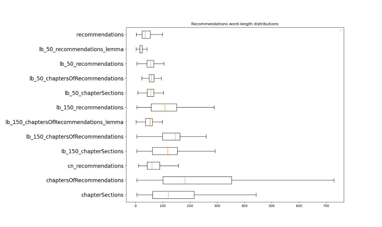
Modelling approaches
Word vectors (bio-embedding intrinsic)
The bio-embedding intrinsic model is trained using the word2vec algorithm on PubMed data, hence we will also be referring to it as bio-word2vec. This was the best performing model during phase 1 amongst several others like Word2Vec, TF-IDF, GloVe and doc2vec (table 1). We need to mention that, at that stage, BERTs were not widely available as BERT was released mid-way through the project. Hence, the BERT models were mainly evaluated on phase 2.
Initial attempts with this model averaged the word vectors of each recommendation document. By “recommendation document”, we refer to either a single recommendation document or a merged recommendation document in the case of a load-balanced dataset. We then hypothesised that including all the words in a document could skew the vectors – the “signal” words would become averaged out with “noise” words. Our next idea was to keep only the nouns from every document, as we thought that those would be the strongest features in each document, and average those instead of the whole document. The results were consistently better using this technique, hence we settled for it. Finally, this model was working best when using the load-balanced set of documents with a threshold of 150 and at a chapter-of-sections level (tables 1 and 2).
BERT and friends
The BERT language model (and related transformer models) triggered a step-change in natural language processing and triggered a whole new family of language models (BERT, RoBERTA, ALBERT, StructBERT, et al). These models are initially trained on massive datasets (such as the 2.5G word English Wikipedia dataset and 800M word BooksCorpus) and then made available. The models can then be refinement trained to perform specific tasks.
One task-specific refinement is Semantic Textual Similarity (STS), part of the SemEval benchmark suite. With BERT, two tokenised sentences are supplied, which are then compared by BERT. BERT responds with a score from 0 to 5, semantically different to the same meaning. However, to compare a sentence against N other sentences, this means we must compute N passes through BERT, which is relatively slow if a CPU is used (minutes rather than seconds). Given that the National Institute for Health and Care Excellence (NICE) prefer not to use specialist hardware (namely, just CPUs), this is not viable.
An alternative approach is to convert the sentence to a vector embedding and then use vector similarity to compare sentences. Unfortunately, BERT is not designed for this – you can add the last layer’s weights as an embedding, but that produces worse results than GloVe.
We also trialled Sentence-BERT, which utilises a Siamese network. This consists of two interlinked BERT networks to generate embeddings directly from sentences. This enabled vector embeddings to be created for each recommendation in advance and stored for late rapid comparison (through, for example, cosine similarity). We used the Hugging Face transformers library, which provides simple, open-source access to many pre-trained models and is used to build Sentence-BERT from pretrained BERT models. We tested the presented models.
Since completing this work, Sentence-BERT has further improved and is now hosted on the Sentence Transformers website. It now includes tutorials on semantic similarity and semantic search, which may be of interest to the user.
Although Sentence-BERT provides a model to embed sentences to n-dimensional vectors, this cannot be used straight out of the box. This is because BERT is used for several mainstream tasks like semantic textual similarity (STS), question answering, General Language Understanding Evaluation (GLUE), for example. To fine tune the BERT weights for a specific task, like STS in our case, sBERT needs to be refine trained. There are two different ways to do so. One is with a natural language inference dataset (NLI), which has labelled sentence pairs with three labels: contradiction, entailment, and neutral. The other is with an STS benchmark dataset, which provides sentence pairs to the Siamese neural network, along with scores ranging from one to five.
Refine-trained Bio-BERT sentence transformers with the Med-NLI and MedSTS datasets
We tried several medical-domain-specific BERT models trained with PubMed data and/or clinical discharge notes. These models would not work well out of the box, for reasons explained previously, but once refined, they could be trained with medical natural language inference (NLI) datasets and med-sts datasets that we obtained from MIMICII and Mayo Clinic respectively. We also obtained BIOSSES [14] and fused it with medical NLI, which gave us slightly better results. Both our fused NLI and STS datasets were small (just 500 records of the fused NLI and 1380 of the med- STS), hence we feel that the results we demonstrate by refine train medical sBert variants could be improved by larger datasets created in the future.
Bio-embedding augmented TFIDF
In this approach, the frequency of words or phrases (terms) in each recommendation are counted to form a recommendation – term count matrix (term frequency TF). The term column values in this matrix are then adjusted according to how rare each term is in the overall corpus of recommendations, which is known as inverse document frequency (IDF). Similarity between recommendations may then be calculated as the cosine between the normalised recommendation term vectors.
For the results reported here, TFIDF was augmented in two ways. Firstly, the vocabulary of terms, up to five grams, was filtered by Wikipedia article titles. Secondly, the TFIDF recommendation vectors were enriched with up to 10 terms from nearby bioword2vec embeddings (enriched terms weighted at 20% of original terms). Other operations included lowercasing, tokenisation, and removal of stop-words (unigrams, bigrams only). The BM25 variant of TFIDF was also employed.
6. Results and discussion
When carrying out the model evaluations, we treated this as a classification problem where, given a particular recommendation, we needed to determine the related recommendations. This means that related is a “positive” result and not related is a “negative” result. We will describe the metrics used for evaluation. Tables 1 and 2 summarise our results for the best performing models.
Metrics used for the benchmarks
Receiver Operating Characteristic
Classifications can be examined with a Receiver Operating Characteristic (ROC) curve, which plots the true-positive rate against false-positive rate. An example is shown in Figure 7.
Figure 7: Example ROC curve demonstrating results coming from the ClinicalBert_dish model (clinical BERT trained with discharge notes). The curve represents the true positive against false positive rate for several similarity threshold cutoffs ranging from maximum to minimum, which are not included in the graph.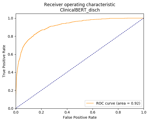
The curve represents the performance of the model when using different thresholds to determine when to assign a result as a “related” (positive) or “unrelated (negative) recommendation. An ideal model would show a curve that is near to the “perfect point” at the top-left of the graph (100% positive results with 0% false positives). The “area under curve” (AUC) summary value for a ROC curve shows 0.5 as a “pure chance” result (represented by the blue diagonal line), with 1.0 being a “perfect” result. A “perfect” result is akin to the probability that a randomly chosen “related” recommendation will be ranked higher than a randomly chosen “unrelated” one. In our case, ROC curves and AUC would represent the ability of the model to rank results by a similarity score. A perfect curve with 1.0 AUC would assign scores to recommendation pairs such that the matching ones would be
Average precision
However, due to our dataset being heavily unbalanced (of approximately twenty thousand recommendations, fewer than 10 will be a positive match), the ROC curve can be overly sensitive to changes in the small number of correct predictions. As a result, our ROC curve may present an overly optimistic view of the performance. A precision-recall (PR) curve was presented to help detect this, plotting precision, which is true positives / (true positives + false positives), versus recall, which is true positives / (true positives + false negatives). The curve is created for a range of increasing thresholds, not visible to the graph, similar to ROC curves. An example is presented in Figure 8.
Figure 8: Example precision-recall curve for the same model we used for the ROC curves above (ClinicalBERT_disch). The curve represents precision versus recall at increasing matching thresholds (not shown in the graph).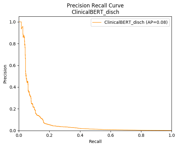
The precision-recall curve can be summarised with “average precision” (AP). Note that, compared with a reasonable ROC curve and AUC score, the PR curve drops off very rapidly with recall, producing a low AP. This helped us recognise when models were not as strong as the AUC first suggested.
Weighted mean reciprocal rank
Finally, as we are performing an information-retrieval task, we used a range of ranking metrics that would reward high-ranked results throughout the experiments samples.
Specifically, Top N is how many related recommendations were returned in the top 200 similarity scores, and Top N recall is calculated as how many related recommendations were in the top 200 divided by the total number of related recommendations. N was chosen to be 200 as this was demonstrated by NICE to be a manageable number of results to review.
Another metric worth looking at is the mean reciprocal rank, which gives us a score of the ranking ability of the model for the whole corpus. We decided to use a weighted mean reciprocal rank to account for the fact that our queries varied in the number of true positives assigned to them; hence, the formula for our metric was: \( \)
$$ WMRR = \frac{1}{Q} \sum_{k=1}^{Q} \left( \frac{1}{n}\sum_{i=1}^{n} \frac{1}{rank_i} \right) $$
Where Q is the number of sample queries, n is the number of samples on our dataset and rank_i is the rank of the true positive i.
Results
Phase 1
We now present our top results from phase 1 (“National Institute for Health and Care Excellence (NICE) standard”) in Table 1, sorted by Top N. “NICE standard” consists of 246 TPs out of 74 sample queries. The record in bold (bio-embedding intrinsic, with the 150 CoR nouns only – lemmatized data processing) was the best performing model at the time, which we forwarded to domain experts for manual investigation of its results.
Table 1 Phase 1 (“NICE standard”) shows results for a selection of our best models, sorted by Top N. Data augmentation (“Data Aug”) notes how we adapted the data before processing, namely N=Nouns only, L=Lemmatized, and S=Stemmed. “LB” is Load Balancing, and 150 CS means Chapters Sections were merged with a target word count of 150. Similarly, CoR is Chapter of Recommendations, whereas CN means context added.
| Model | Data Aug | AUC | Mean Prec | WMRR | Top N | Top N Recall | Load Balancing |
| Bioembedding Augmented TFIDF | CN | 0.943 | 0.067 | 0.156 | 141 | 0.573 | – |
| Bioembedding Augmented TFIDF
|
– | 0.942 | 0.083 | 0.172 | 138 | 0.561 | – |
| micros_sbert_refined_sts | CN | 0.93 | 0.06 | 0.115 | 133 | 0.54 | – |
| bio_embedding_intrinsic | CN N L | 0.931 | 0.02 | 0.102 | 122 | 0.496 | – |
| GloVe-840B-300d | CN N | 0.913 | 0.018 | 0.108 | 119 | 0.494 | – |
| BERT-large-uncased | CN N L | 0.883 | 0.031 | 0.064 | 115 | 0.467 | – |
| GloVe-6B-300d | CN N | 0.915 | 0.013 | 0.076 | 114 | 0.463 | – |
| GloVe-42B-300d | CN N | 0.924 | 0.012 | 0.088 | 113 | 0.459 | – |
| BioWordVec pubmed MIMIC III | CN N L | 0.935 | 0.019 | 0.099 | 111 | 0.451 | – |
| BERT-base-uncased | CN N L | 0.863 | 0.032 | 0.076 | 111 | 0.451 | – |
| bio_embedding_intrinsic | – | 0.899 | 0.012 | 0.056 | 111 | 0.451 | 150 CoR |
| Biobert v1.1 pubmed | CN N L | 0.887 | 0.042 | 0.104 | 107 | 0.435 | _ |
| BioWordVec pubmed MIMIC III | CN N L | 0.887 | 0.025 | 0.091 | 106 | 0.431 | – |
| Biobert v1.1 pubmed | – | 0.896 | 0.024 | 0.085 | 102 | 0.415 | – |
| bio_embedding_intrinsic | – | 0.857 | 0.012 | 0.044 | 97 | 0.394 | 150 CoR |
| BERT-base-uncased | – | 0.849 | 0.023 | 0.054 | 89 | 0.362 | – |
| BioWordVec pubmed MIMIC III | – | 0.836 | 0.011 | 0.032 | 82 | 0.333 | 150 CoR |
| GloVe-42B-300d | – | 0.811 | 0.024 | 0.087 | 68 | 0.276 | – |
| GloVe-6B-300d | – | 0.806 | 0.021 | 0.079 | 64 | 0.260 | – |
| NICE | – | N/A | N/A | N/A | 277 | N/A | N/A |
Note that we have recorded the base and top scores for each model, where the base score is the raw recommendations, and the top score from all variants of load balancing, grouping and context addition. Interestingly, context-added variants were better than all forms of load balancing in this table.
Phase 2
Additional labels were provided by the National Institute for Health and Care Excellence (NICE) as part of phase 2 (using potential additional true positives flagged by bio_embedding_intrinsic), forming the “Gold Standard”, which consisted of 875 TPs in total out of 74 queries in total. The models were then re-run and top results presented in Table 2. Results are again sorted by Top N, using the same naming convention as Table 1.
Table 2 Phase 2 (“Gold standard”) shows results for a selection of our best models, sorted by Top N. Data augmentation (“Data Aug”) notes how we adapted the data before processing, namely N=Nouns only, L=Lemmatized, and S=Stemmed. “LB” is Load Balancing, and 150 CS means Chapters Sections were merged with a target word count of 150. Similarly, CoR is Chapter of Recommendations, whereas CN means context added.
| Model | Data Aug | AUC | Mean Prec | WMRR | Top N | Top N Recall | LB |
| bio_embedding_intrinsic | N L | 0.932 | 0.091 | 0.181 | 702 | 0.802 | 150 CoR |
| Bioembedding Augmented TFIDF | CN | 0.980 | 0.275 | 0.231 | 675 | 0.771 | – |
| BioWordVec pubmed MIMIC III | N L | 0.933 | 0.090 | 0.173 | 674 | 0.770 | 150 CoR |
| Bioembedding Augmented TFIDF | – | 0.977 | 0.255 | 0.206 | 650 | 0.743 | – |
| micros_sbert_refined_sts | CN | 0.96 | 0.21 | 0.226 | 641 | 0.732 | – |
| micros_sbert_refined_sts |
– |
0.97 | 0.13 | 0.167 | 633 | 0.723 | 150 CoR |
| micros_sbert_refined_sts_x_sentsplit | CN | 0.96 | 0.05 | 0.157 | 618 | 0.706 | – |
| dmis_bio_nli_fused | – | 0.97 | 0.17 | 0.155 | 600 | 0.686 | 50 CoR |
| bio_embedding_intrinsic | CN | 0.936 | 0.116 | 0.203 | 583 | 0.666 | – |
| GloVe-840B-300d | N L | 0.904 | 0.083 | 0.163 | 583 | 0.666 | 150 CoR |
| BioWordVec pubmed MIMIC III | CN N | 0.935 | 0.073 | 0.198 | 573 | 0.655 | – |
| bio_embedding_intrinsic | – | 0.906 | 0.087 | 0.165 | 564 | 0.645 | 150 CoR |
| micros_sbert_refined_sts_x | – | 0.95 | 0.07 | 0.171 | 561 | 0.641 | 150 CoR |
| BioWordVec pubmed MIMIC III | N L | 0.911 | 0.065 | 0.169 | 548 | 0.626 | 150 CoS |
| GloVe-840B-300d | CN | 0.897 | 0.077 | 0.194 | 522 | 0.597 | – |
| microsoft biobert | – | 0.890 | 0.116 | 0.116 | 506 | 0.578 | – |
| Biobert v1.1 pubmed | – | 0.926 | 0.062 | 0.108 | 506 | 0.578 | – |
| WordCount | N S | 0.953 | 0.071 | 0.159 | 503 | 0.575 | 150 CoR |
| GloVe-840B-300d | – | 0.860 | 0.063 | 0.154 | 496 | 0.567 | 150 CoR |
| GloVe-840B-300d | N L | 0.878 | 0.045 | 0.125 | 495 | 0.566 | – |
| GloVe-840B-300d | N | 0.878 | 0.042 | 0.126 | 485 | 0.554 | – |
| ClinicalBERT_disch_20200120 | – | 0.916 | 0.081 | 0.102 | 481 | 0.550 | – |
| scibert_scivoca | – | 0.907 | 0.060 | 0.100 | 470 | 0.530 | – |
| bio_embedding_intrinsic | – | 0.870 | 0.065 | 0.127 | 462 | 0.528 | – |
| BERT-large-uncased | – | 0.881 | 0.083 | 0.144 | 410 | 0.469 | 150 CoR |
| BioWordVec pubmed MIMIC III | – | 0.857 | 0.059 | 0.125 | 410 | 0.469 | – |
| BERT-large-uncased | – | 0.884 | 0.055 | 0.093 | 396 | 0.453 | – |
| BERT-base-uncased | – | 0.890 | 0.051 | 0.083 | 395 | 0.451 | – |
| GloVe-840B-300d | – | 0.814 | 0.039 | 0.122 | 397 | 0.454 | – |
| ALBERT xlarge v2 | – | 0.796 | 0.058 | 0.135 | 328 | 0.375 | 150 CoR |
| ALBERT xlarge v2 | – | 0.793 | 0.020 | 0.068 | 308 | 0.352 | – |
| NICE | – | N/A | N/A | N/A | 277 | N/A | N/A |
Discussion
The results in table two show the best models sorted by their performance in the top-200 ranked results. Also, we have used bold to highlight numbers models that performed at the top in other areas like mean reciprocal rank. There are a few remarks to make on the results of table two.
The bio-embedding intrinsic appears to be the best performing model, but we must take into consideration that this model’s results have been manually evaluated by domain experts, hence all its true positives in the top-200 ranks have been revealed. This is not the case for all other models as there is a likelihood that many unknown true positives are hiding in their top-200 ranked results. Table 1 results, which were produced for that purpose, show that several models like the refine-trained sentence bioBERT and the augmented TFIDF model performed better on the phase 1 the National Institute for Health and Care Excellence (NICE) standard. However, these models were not available at phase 1 as BERTs were invented at a later stage and the augmented TFIDF technique, as well as the context-added data augmentation method, were discovered during phase 2.
With that in mind, our recommendation is that Augmented TFIDF and Microsoft’s sentence BERT, which is refine trained with medical NLI and STS data, should not be underestimated. Especially for the latter, we saw a big improvement in scores when training it with medical NLI and STS data. It feels as if the NLI and STS datasets we had in hand were small, but when larger medical datasets will be available then of course there should be another evaluation of the model.
Models were evaluated as a combination of all the metrics in the tables. This helped to overcome the question of whether the top n metric might be sensitive to the number of true positives in each query. Data load balancing and augmentation is something that worked very well, as demonstrated through our benchmarks with all our top-20 model results in the table having used either load-balancing or context-enhancement variants of the data.
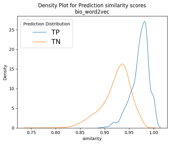
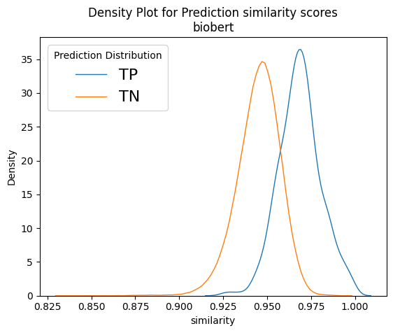
Considering the results in Tables 1 and 2 and their running times, we concluded that our best models were the refine-trained bio-sBERT (both as sentence transformers and cross autoencoders) and the bioword2vec ones (bioembedding intrinsic and MIMIC III models). We decided to test these further by looking more closely at some normalised density plots for these models run with the context-added augmentation method.
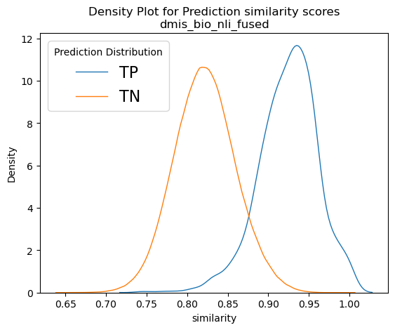
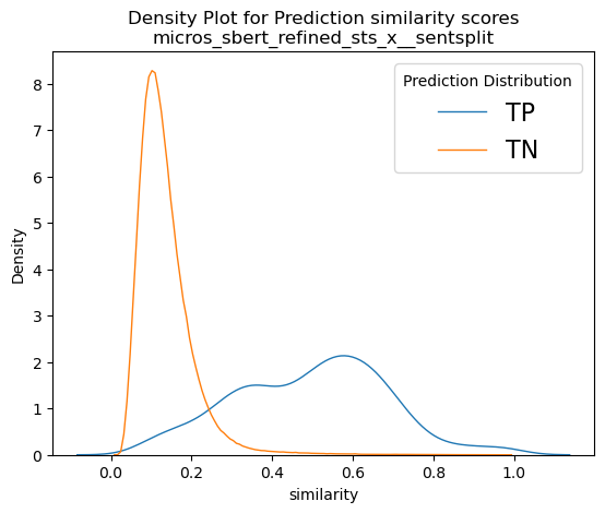
Figure 9 depicts normalised density plots for the similarity scores found in true positives and true negatives. The plots were normalised as there was a difference in magnitudes for the two curves as the true negatives account for almost the whole corpus. The plots come from two of our best models, namely bioword2vec and several variants of bioBERT. We can see that in all plots a large part of the orange curve overlaps the blue. If we consider that the total for the orange curve is approximately 20,000 recommendation documents, it is apparent that, if we wished to recover most of the known true positives, we would have needed to include thousands of true negatives too in our results, which is rather impractical. That goes to show that, although our models have almost doubled NICE’s capacity to recover linked recommendations, there is still plenty of room for improvement and plenty of potential for better models to be uncovered in the future!
Taking a closer look at Figure 9, we can see that the score distributions of refine-trained variations of BERT at the bottom row look less overlapping and their peaks are more spaced apart. It is also interesting to see the Cross-encoders distributions on the bottom right-hand plot. It seems that the true negative scores are well distributed in the range of values [0,3], but true positives span the whole spectrum of values between zero and one with enough overlap on the TN curve. In theory, cross encoders should be performing better than sentence encoders when both are refine-trained, but we did not see that in our case. However, cross encoders are significantly slower than sentence transformers (>10x slower), and their training and evaluation would not allow as much experimentation as we could do with other models because of time constrains. Our intention was to explore the possibility of using the sentence transformer models to shortlist 1,000 – 2,000 recommendations and then use cross encoders to re-rank them. But since we did not get the significantly better results that we expected, we dropped the idea, but that prospect should be revisited in the future.
Figure 9: Example normalised density plots – on the top left the word2vec model and on the top right a non-refine trained biobert model. On the bottom left, a refine-trained dmis bio-bert model using sentence transformers and on the bottom right a refine-trained on nli and sts biobert cross-encoder model. The blue curves represent true positives and the orange ones the true negatives.
7. Deployment of the proposed method
Outline of proposed proof of concept
The model assessed as the best performing to meet the National Institute for Health and Care Excellence’s (NICE) needs was the bio_embedding_intrinsic using the lemmatized nouns only chapter of recommendations at 150 words level. The reason for this choice was that BERTs would need a GPU to execute at reasonable pace, and the TFIDF augmentation method was not developed at the time. Also, this model could be used out of the box for keyword to recommendation searches too. A sentence BERT would not function as well with an input of one or two keywords as sentence transformers were not built for that purpose. The next step was to produce a proof of concept that would be deployed on NICE infrastructure and allow users to interact, query and make use of this method.
The proposed implementation of the proof of concept is as follows:
- Package core methods that came out of the methodology and model comparison into a set of python functions as part of a package that then will underpin the server defined in point 2.
- Create a python web server able to process incoming requests containing keywords or recommendation IDs and able to then use the chosen machine-learning model (as well as an index of all recommendations) to predict nearest matches. This can serve as both an API for direct programmatic access as well as a back end for a more usable UI.
- Create a UI that allows colleagues in NICE to input recommendation IDs and keywords, which then will get sent to and processed by the server described previously. This UI also then displays the response containing all the matching recommendations to the user.
Therefore, it follows a similar pattern to the “model view controller” pattern, where the server is the model underpinning the logic, and containing the machine-learning model element, and the UI is then both the controller and the presentation layer. Figure 10 illustrates the proposed interactions:
Figure 10: Simplified diagram of the final interactions between the UI and Norma. Norma sits as the underpinning library for the server, and the server works to enable the translation between the user interface and Norma.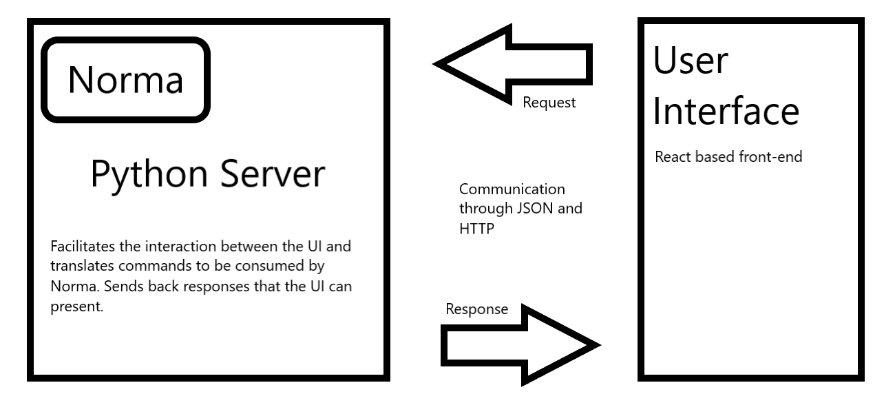
A simplification of the outlined proposal can be achieved by merging the python server and the python package steps into one step (and consequentially one codebase). However, the decision was made to keep them separate to allow greater modularity when deploying on the users’ infrastructure and to allow easy in-place replacements of either component because of minimal coupling.
Implementation details
After consulting the National Institute for Health and Care Excellence (NICE) on the previous outline for a proposed proof of concept, work started to implement the distinct parts. Each part was split into a separate repository prefixed by the project name (norma, norma-server and norma-ui).
8. Python package (Norma)
To develop the python package, the experimental code developed as part of the model benchmarking exercise was assessed and relevant parts extracted, reviewed and refactored. The package was then documented, core parts of it were tested and this was fed into the next stage of work – creating the server.
Server
The server was built in python using flask as the main tool to translate HTTP requests into python commands. The implementation and codebase are fairly lightweight, consisting of mainly one API endpoint that is able to accept post requests with a given JSON body containing all the information required to find matching recommendations.
It is worth noting that for the server to provide matches it needs to have a dataset of recommendations that will serve as the core look up for any recommendation-matching requests. This means that, upon starting the server, a dataset and model are loaded into memory, and these two components are key to the process of providing recommendation matches. Note that, upon delivery of the proof of concept to NICE, the data was loaded from static files. However, it was built in a way that would allow the end user of this server to tweak the ingestion functions so that these data could be drawn from a database instead. This would allow the decoupling of the server and the recommendation in the future which, in turn, would provide matches that were always up to date.
The core of the server is one web endpoint performing the translation of requests to the python code. This endpoint expects a POST request with a body similar to the following JSON snippet:
{
“query”: [“keyword1”, “keyword2”, “…”],
“type”: “keywords”,
“topn”: “200”,
“threshold”: “0.98”
}
Each field parametrises the python code and dictates the results that will be sent back. Namely, the type parameter switches between exact word search across documents, semantic keyword matching and recommendation-to-recommendation matching. The “query” then contains either the keywords required for exact or semantic keyword matching or a string containing the recommendation ID in the case of recommendation-to-recommendation lookups. The “topn” and “threshold” parameters dictate how many maximum results to return and what the lowest score is to return.
The response is then of shape:
[
{
“rec_id”: “CG104.4”,
“score”: 0.32,
“text_snippet”: “Some text from the recommendation”,
“guidance_title”: “Vitamin d…”
},
…
]
Simply put, it will contain a list where each entry is a recommendation that matched against the specific query and some other metadata and sample text.
UI
The final component of the deployed Norma is the presentation and interaction UI, which would allow users to send queries and view the results. This component was built as a single-page React.js application. It does not use any formal state management, like Redux, and is fairly simple in its features.
To expedite the process of building the proof-of-concept UI, the popular Material UI framework was chosen to provide components such as buttons, bars and inputs. Using these components, a simple layout consisting of a single input field and a few customisation options was built (see Figure 10 A screenshot from the NORMA interface). This allows users to provide either keywords or recommendation names in the input and set a few parameters. All these inputs simply correspond to the API specification show above and are passed on to the server upon submission.
There were a few challenges to overcome, mainly because of specific stakeholder requirements relating to the user experience. That said, most of these were trivial to solve and were mainly focused on things such as making the input box more accepting of varying ways to input recommendation IDs.
Figure 11: A screenshot from the NORMA interface.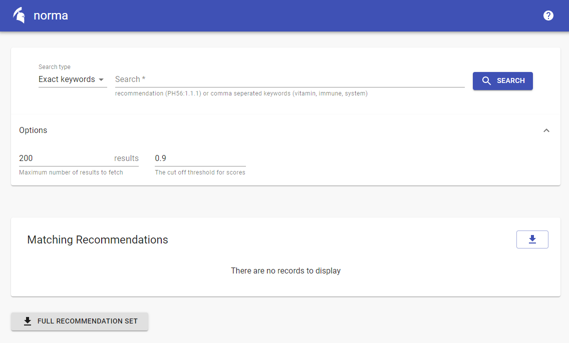
NORMA live
The National Institute for Health and Care Excellence (NICE) formally launched NORMA across the organisation in February 2021. Its use has since expanded beyond the original use case, to support guideline scoping activity and to respond to external enquiries. Prior to launch, the digital team at NICE also made changes to accommodate additional guideline structures. Specifically, the text engineering pipeline was updated to enable the capture of recommendations from new coronavirus (COVID-19) guidance, which was structured very differently to previous guidance. NICE were also able to capture some older recommendations that had been overlooked until recently because of their unique content structures. Further improvements were made to the UI to make it easier and more convenient to use. Most notably, the entire live recommendations dataset was made available as a download to allow more widespread use and analysis across the organisation in a way that had never been possible before. Finally, Google and Hotjar tracking were added to support usage analysis.
9. Conclusions
This report summarises our efforts to improve the National Institute for Health and Care Excellence’s (NICE) surveillance operations using state-of-the-art data science and natural language processing (NLP). The project outcomes were successful and that was evident even at early stages of the project when our initial results brought a 2.5x improvement in accuracy over the existing surveillance at the time. In addition, it reduced the time lag of finding related recommendations from weeks to hours. This means that updates in healthcare recommendation can now be addressed by NICE without the previous week-long time lag. Given the ease and speed of use, significantly more updates can also be done in a given timeframe, which in turn would reduce any potential backlogs significantly. This is not only good for NICE’s operations but for the public in general.
Recommendation for use and future improvements
Our recommendation is that the National Institute for Health and Care Excellence (NICE) uses the new tool in such a way that it can accommodate future improvements. Natural language processing (NLP) is fast evolving and a two-to-three-yearly tech refresh on models would be a good option. The top-200 results coming out of queries could be scored by experts in such a way that there is a score between 1.0-5.0 between recommendation pairs, along with a label (entailment, contradiction and neutral) on the returned Excel files. This way, NICE can build a domain-specific training sample to refine train sentence transformers in the future, either on its own or fused with the existing ones we hold.
There have been discussions between DSC and NICE with regards to what happens with the unique recommendation IDs when there is an update. Our recommendation is that there should be a new Boolean field added to the JSON structure <live>, which will be true if the recommendation is live and false if not. New recommendations will then be assigned a new unique ID by simply incrementing the last available ID number by one. For example, if the recommendation of product x, with ID 1.2.6.13, is replaced by a new one, and the last ID of the recommendations section was 1.2.6.18, then the recommendation that replaces 1.2.6.13 would get an ID of 1.2.6.19 and its <live> switch would be assigned a true value, whereas the 1.2.6.13 recommendation’s <live> Boolean would be turned to false. This way, NICE will also keep a good track of the history of its dataset, and of course more data will be available to train new models in the future.
Concluding comments
NORMA is being actively used across the organisation and its use case is beyond that which it was originally developed for. For example, it has supported the scoping of new guidelines to ensure there is no duplication of existing work, and it allows for quicker querying of recommendation content to answer public enquiries.