Data science for the public good

The Sustainable Development Goals (SDGs) have been developed by the UN as a “blueprint to achieve a better and more sustainable future for all”; they are designed to end poverty, halt climate change and reduce inequalities. The SDGs are made up of 17 goals and 244 indicators, making the mandate placed on countries to report on the SDGs a huge challenge. The Office for National Statistics (ONS) reports the UK data for the SDG indicators on the UK SDG data website.

One of the indicators that has, until now, remained unreported for the UK is indicator 6.6.1: Change in the extent of water-related ecosystems over time. It focuses on water-related ecosystems that provide an important service to society, including open waters (rivers and estuaries, lakes and reservoirs), wetlands (peatland and reedbeds) and groundwater aquifers.

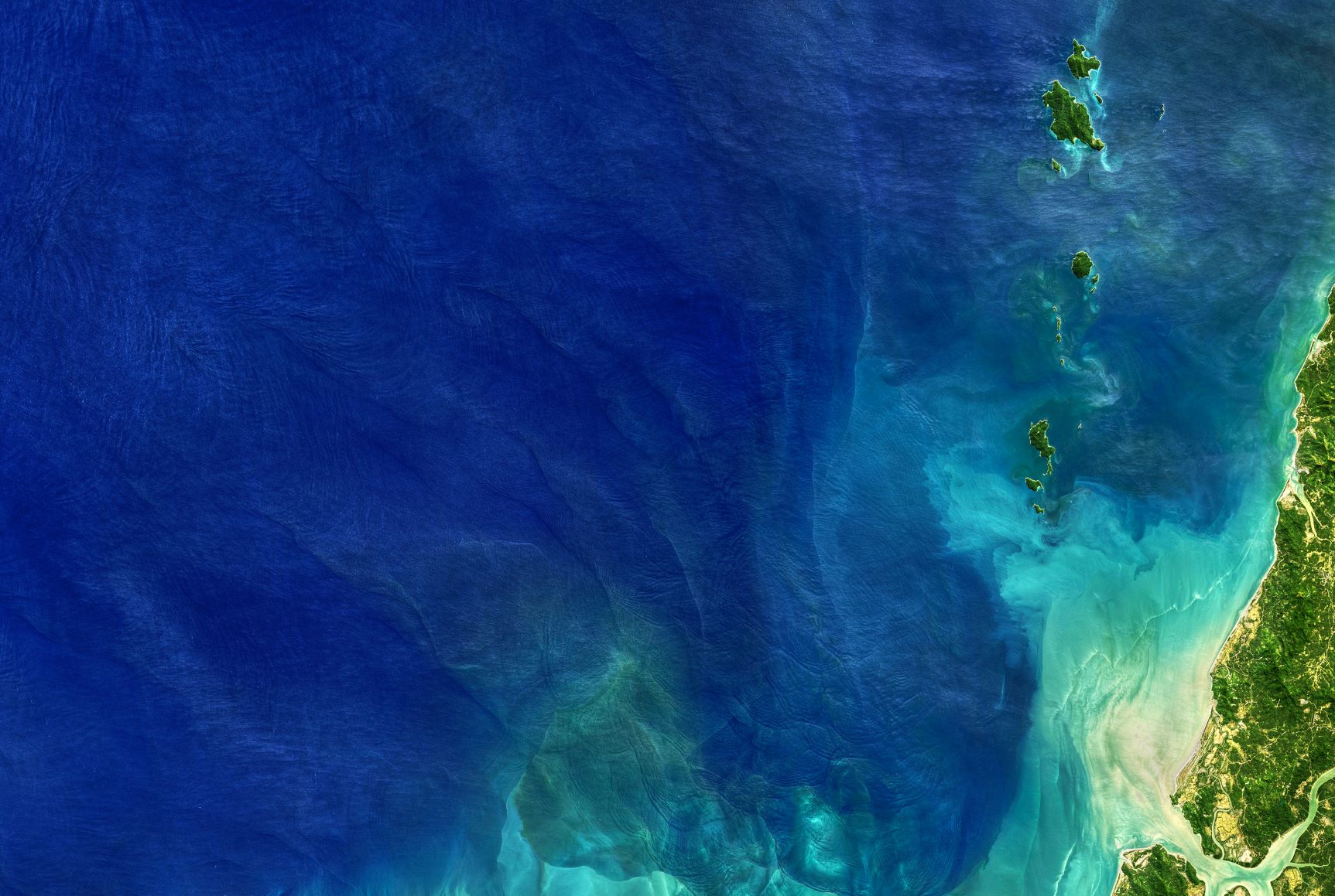
Recognising a global need for better data to measure this indicator, the Joint Research Centre and Google have developed the Global Surface Water Explorer (GSWE) dataset. This is based on satellite imagery from the past 35 years and measures changes in the distribution of inland open water, for example, lakes and reservoirs, a sub-indicator of 6.6.1.

In this blog, we describe how we have assessed the quality of this novel data source to better understand its value and fitness-for-purpose, and then produced data that report the UK’s position on indicator 6.6.1.

Data sources and function

The Global Surface Water Explorer (GSWE) was developed specifically to help countries report on indicator 6.6.1, recognising the lack of available data sources that monitor changes in both permanent and transient water. It was developed in partnership with the UN Environment Programme (UNEP), the European Commission Joint Research Centre and Google. The GSWE dataset, built using a peer-reviewed consistent methodology, is global and publicly available, for example, via the Google Earth Engine.

The GSWE tool quantifies monthly changes in global surface water since 1984 at 30-metre pixel resolution using around 3 million Landsat satellite images. It records the months and years when water was present, where occurrence changed and what form changes took in terms of seasonality and persistence. It classifies three different water types:

• permanent water: an area that is underwater throughout the year
• seasonal water: an area that is underwater for less than 12 months a year
• ephemeral water: an area that is episodically underwater in different years

We applied a number of processes to transform the imagery data from the GSWE into tables and maps that are reported via the UK Sustainable Development Goal (SDG) national reporting platform. These processes include constraining data to official high-water mark boundaries, which helps ensure that coastal water is not included in measures and mitigating the impact of persistent cloud cover.

You can read more about the methods used to produce these data in the quality and methodology report we have produced as part of our commitment to voluntarily apply the Code of Practice for Statistics to our non-official outputs. This helps to provide transparency and improve the reporting capability of other National Statistical Institutes. The code for performing data extraction from Google Earth Engine and the computation of statistics for different geographic areas are available on our GitHub pages.

Data quality

As of November 2020, the Sustainable Development Goal (SDG) team at the Office for National Statistics (ONS) reported that the UK has published headline statistics against 80% of indicators. Often, indicators do not align with national data collection strategies, so innovative solutions and novel data sources such as global, open and geospatial datasets are increasingly being explored. The approach taken for this indicator (6.6.1) differs from methods traditionally used to capture water for topographic mapping, where trained surveyors measure the boundaries of every individual water feature either in the field or using very high-resolution aerial photography. The Global Surface Water Explorer (GSWE) data are not official statistics, so we opted to voluntarily review the dataset for the purpose of UK SDG reporting against the quality framework of the Code of Practice for Statistics. You can read more about the quality analysis in the quality and methodology report.

The main strengths of the data are that they have been produced by water experts at the UN Environment Programme (UNEP) and European Commission Joint Research Centre specifically to monitor this indicator. The methods used to produce the data are comprehensively described and peer reviewed, and the accuracy of the model is high. Tested against 40,000 samples, it is estimated the model produces less than 1% false-positive detections of water and less than 5% false negatives. Furthermore, the data are open and available for the entire world and can therefore be compared internationally. This aligns with our work to support colleagues across the world to develop their capability.

In using the GSWE data source certain quality trade-offs have had to be made. We favoured the ability to measure changes comprehensively over space and time instead of the highest spatial resolution. Spatial accuracy is related to the resolution at which the satellite imagery being classified was captured at, below which water features will not be detected. These data used Landsat imagery with a pixel resolution of 30m (900m²), which means that we do not have data for smaller water bodies (including small lakes, rivers and streams). In addition, the tool currently only gives data on open water, which cannot yet be separated into natural water bodies (for example, lakes) and man-made water bodies (for example, reservoirs).

Measuring spatial extent

Using the source data, the presence of different types of inland surface water (permanent, seasonal and ephemeral) each year between 1984 to 2019 can be identified at the level of 30m pixels. Spatial extent is calculated by aggregating pixel counts from this level to HydroBASINs, which are a series of polygon layers that depict watershed boundaries at a global scale. The HydroBASINs use the Pfafstetter coding system, which allows for analysis of catchment topology. Catchments can be broken down further into smaller sub-basins; with each subdivision, the Pfafstetter level increases. Here, a Pfafstetter level of six was used, giving us data for 38 catchments across the UK. Figure 1 shows the 2019 data on the extent of different types of surface water aggregated by HydroBASIN.

Figure 1: Spatial extent as a percentage of land area of different types of surface water aggregated to HydroBASINS in the UK in 2019

Source: Global Surface Water Explorer data; European Commission Joint Research Centre; and Google

Notes:

1. Data scales vary.
2. The Vega-Lite code for visualisations is available on the GitHub repository.

Scotland accounts for most of the UK’s surface water. From 1984 to 2019, 50% of the UK’s permanent inland water occurred in Scotland, while Northern Ireland contained 31% and England and Wales together only contained 19%. Figure 1 shows that the HydroBASIN with the greatest spatial extent of permanent water fell in Northern Ireland, which contains Lough Neagh, the UK’s largest lake by area. That HydroBASIN accounts for 66% of Northern Ireland’s permanent inland waters. Conversely, England held an average of 57% and 43% of all ephemeral and seasonal inland waters, from 1984 to 2019. Wales contributed the least to each water type nationally: 5% seasonal and 3% ephemeral and permanent inland surface water, not including rivers and estuaries.

Measuring change in extent

Comparing spatial extent of each water type between years allows the second part of the sub-indicator, percentage change in spatial extent, to be calculated. The change in extent, described using the indicator’s monitoring methodology is calculated as:

\(\)
\( \text{Percentage Change in Spatial Extent} = \frac{\text{γ – β}}{\text{β}} \)

where:

β = the average national extent from 2001 to 2005

γ = the average national extent of any other five-year period

Figure 2 shows that the source data contains two periods of anomalous data: 1991 to 1997 (excluding 1994) and 2004 to 2008. These are because of a lack of suitable Landsat images from which to derive water measurement, likely a result of persistent cloud cover. The base period of 2001 to 2005 includes the anomalous years 2004 and 2005. To mitigate the impact of variable cloud cover, we have taken the modal value of each pixel across the baseline years to calculate the average spatial extent per HydroBASIN (β). Further details on the source data and mitigating the impacts of these anomalous periods is provided in the quality and methodology report.

Figure 2: Annual national extent of inland surface water separated by type (permanent, seasonal and ephemeral)

UK, 1984 to 2019

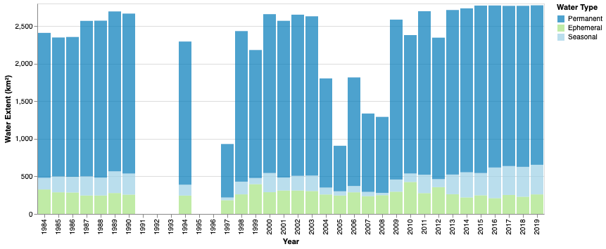
Source: Global Surface Water Explorer data; European Commission Joint Research Centre; and Google

The code performing Google Earth Engine extraction and zonal statistics is available on the Data Science Campus’ GitHub.

Coherence with other data sources

The extent of permanent water bodies in Great Britain is captured by the Ordnance Survey, but these data lack the time series provided by the Global Surface Water Explorer (GSWE). We have compared the coherence in locations of water between the two data sources, after having (approximately) accounted for differences in spatial resolutions. We identified errors of commission and omission of around 2% by area, though much of this can also be accounted for in terms of the approximations required to make the datasets a comparable resolution. A very small number of notable anomalies were identified related to artificial waterbodies, for example, a dockyard. Such occurrences were rare and within the stated accuracy levels of the source data.

The UN Environment Programme (UNEP), European Commission Joint Research Centre and Google partnership recently released the Freshwater Ecosystems Explorer. This uses a similar methodology using the GSWE dataset and is able to estimate unobserved permanent and seasonal water. We have compared results using the method outlined earlier with those from that source and found less than 1% difference for seasonal waters and approximately a 2% difference for permanent water extent. The discrepancies likely arise from the use of a more generalised boundary – Global Administrative Unit Layers (GAUL) – when processing GSWE data, which means seawater is being included at coastal margins. The data we present through the UK Sustainable Development Goal (SDG) reporting platform has been aggregated against the high-water-mark national boundaries produced by Ordnance Survey. This limits the misclassification of seawater and provides consistency in the standard approach for compiling National Statistics.

Insights from novel data sources, such as satellite imagery open exciting new possibilities for monitoring the SDGs. However, in using new data sources we must be sensitive to the different issues that arise in the collection and production of such data. In this work, we have applied the principles of the Code of Practice for Statistics to assess the concerns and their impact on the fitness-for-purpose of the indicators produced. While the Code was not expressly developed for such data sources, we have nonetheless found it to be an excellent framework to help guide assessments and reporting of the quality of data science products.