Generative adversarial networks (GANs) for synthetic dataset generation with binary classes
One thing almost all of us could agree on is that we would all like easier and unrestricted access to good-quality data in various spheres of our lives. Good quality data (like oil) are valuable, however it’s not always available, no matter how deep you drill. In most cases, fit-for-purpose real-world data generation can be difficult, expensive, time-consuming, or simply not possible, and the real data are almost always vulnerable to data privacy breach incidents.
In this work we propose to use synthetic data generation methods to produce substitute data closely resembling real data in data-limited situations, minimising the need for accessing real data to make informed decisions. Specifically, we propose to use generative adversarial networks (GANs), which are a type of neural network that generates new data from scratch. GANs feed on random noise as input, and as the training progresses it can produce realistic (synthetic) copies of the real data. GANs have been found to discover structure in the data that they have been trained on, which is remarkable if the underlying data structure or pattern is not evident to us mortals and/or difficult to pull it out with other techniques.
Our goal is to generate synthetic versions of a dataset with binary classes using four different variations of GAN architectures. As an exploratory dataset we will use a freely available admin dataset (with both numerical and categorical features) and will use different GAN models to generate its synthetic copies. It is worth noting that the findings of our GAN models could be easily generalised to other datasets with similar data structures. We will show that using GANs it is possible to produce synthetic copies of our chosen dataset that are close to the original dataset for a variety of real-world applications. Furthermore, we will use a range of techniques to assess the quality of the generated synthetic data.
1. Main findings
Synthetic data are a powerful tool when the required data are limited or there are concerns to safely share it with the concerned parties. When data privacy is a requirement and the generated data are prone to attacks from sophisticated attackers with lots of computational power, we recommend the use of generative adversarial networks (GANs) possibly in conjunction with privacy-preserving mechanisms such as differential privacy.
We have used four different GAN architectures to generate synthetic copies of the US adult census dataset with binary classes, which is a freely available open dataset with binary classes, which is a freely available open dataset extracted from the US census bureau database.
The quantitative results from our experiments on synthetic data generation with several methods suggest that our framework is capable of producing high-quality synthetic samples as the Pearson correlation structure of the real data was closely reflected by the correlation structure of the synthetic data. This indicated that relations between the variables in the original data are preserved in the synthetic data. Different GAN architectures differ in the quality of the generated synthetic data, where one specific architecture Wasserstein distance (WGAN) is shown to give the best performance.
One of the most appealing applications of synthetic data generation is data augmentation. To ensure our generated synthetic data has a high quality to replace or supplement the real data, we trained a range of machine-learning models on synthetic data and tested their performance on real data whilst obtaining an average accuracy close to 80%.
We show that synthetic data generative methods such as GANs are learning the true data distribution of the training dataset and are capable of generating new data points from this distribution with some variations and are not merely reproducing the old (training) data the model has been trained on. We have confirmed this finding using a range of non-parametric statistical significance tests.
Synthetic data generation methods score very high on cost-effectiveness, privacy, enhanced security and data augmentation to name a few. However, synthetic data generation models do not come without their own limitations. While synthetic data can mimic many properties of real data, by their very design the synthetic data generation models we have investigated do not recreate the original data exactly. At the same time, any analysis on synthetic data needs to be verified on the real dataset.
The quality of synthetic data is highly dependent on the quality of the model that created it. The generative models we have focused our attention on can be excellent at approximating the data distribution of the original datasets, uncovering the underlying patterns in the datasets and recognising statistical regularities in datasets, but at the same time they can also be susceptible to statistical noise.
Due to the complexity and varied nature of datasets available to us today, our findings suggest that the best one could hope for is the possibility to generate customised synthetic datasets in the future while not attempting to design a universal synthetic data generation tool. Our findings in this work suggest that even in the situations where it is necessary to generate synthetic data it should always be mixed with reality to make informed decisions.
Overall, the synthetic data generation using GANs is a research intensive field and we are hopeful that further future work on the project and subsequent improvements on the architecture could lead to the generation of high-quality data useful for a variety of applications.
Our next steps will be to further improve the operation of our synthetic data generation models, explore other variants of GANs, explore GANs for discrete data and perform a more quantitative analysis on the quality of the generated data. Eventually, we are working towards making our synthetic data generation framework fit for purpose to produce good-quality datasets for real-world applications, including census and clinical data.
The rest of this article is structured as follows:
- introduction to the working of GANs
- results obtained so far
- some of the limitations of GANs and synthetic data
- short summary and outline for potential future works
2. Synthetic data using GANs
Synthetic data can be broadly identified as artificially generated data that mimics the real data in terms of essential parameters, univariate and multivariate distributions, cross-correlations between the variables and so on. Synthetic data can be created algorithmically. Firstly, by stripping any personal information (names, addresses, postcodes and so) from a real dataset to anonymise it. Another method is to create a generative model from the original dataset that produces synthetic data that closely resembles the real data; it is this later option we choose to explore to generate synthetic data. A class of generative models we choose to pursue in this work learns from large, real datasets to ensure the data it produces accurately resembles real-world data and builds on robust statistical, machine learning and state-of-the-art deep learning techniques. Specifically, we use generative adversarial networks (GANs), a class of powerful deep neural network algorithms to learn to mimic any distribution of data.
GANs were first designed by Ian Goodfellow and have since gained widespread attention in the artificial intelligence (AI) and the wider data science community as they can be trained to create worlds almost identical to our own in practically every possible domain including imagery, music, speech, text and so on. GANs belong to a class of generative models and encompass a powerful way of learning any kind of data distribution based on unsupervised learning. What distinguishes GANs from other synthetic data generation models is that GANs aim to learn the true data distribution of the training dataset with a view to generate new data points from this distribution with some variations and not just reproducing the old data the model has been trained on. Since it is difficult to always learn the exact true distribution of the training data, GANs try to use the power of neural networks to learn a function to approximate the mapping to model a distribution as close as possible to the true data distribution. Recently, opening a lucrative avenue for the AI industry, GANs were used to create the 2018 painting Edmond de Belamy, which sold for $432,500.
Portrait of Edmond Belamy created by a Generative Adversarial Network (a class of deep neural network) and sold for $432,500 at Christie’s. Generative Adversarial Network was one of the methods explored in the data science campus synthetic data generation experiment. Image credit: Christies.com
GANs are not the only synthetic data generation tools available in the AI and machine-learning community. In a complementary investigation we have also investigated the performance of GANs against other machine-learning methods including variational autoencoders (VAEs), auto-regressive models and Synthetic Minority Over-sampling Technique (SMOTE) – details of which can be found in our report “Synthetic Data for public good“. Each method has its respective pros and cons but for the sake of this work we will exclusively focus on various architectures of GANs. Moreover, the scope of this present work is to explore different GAN architectures to produce synthetic copies of real datasets with multiple classes, which was beyond the scope of some of the other architectures (VAEs, auto-regressive models and (SMOTE)) analysed in our parallel investigation.
In the present work, as opposed to using GANs for the generation of images, our motive is to use them for the generation of admin data that has received comparatively little attention from the AI community. Furthermore, we are interested here in using GANs for the generation of datasets with binary classes. We will use different variations of GANs to generate synthetic copies of an exploratory dataset with two classes. For the purposes of testing the performance of our synthetic data models, we will use the US adult census dataset, which is a freely available open dataset extracted from the US census bureau database. The dataset is initially designed for a binary classification problem and the task is to predict whether a person earns over $50,000 a year. It is not balanced and only about 25% of the records in the dataset have a class label of greater than $50,000; this will require us to ensure that proportionate weights are assigned to records from each class proportionally representing the values of “income” column. The dataset is a mixture of discrete and continuous features, including age, working status (workclass), education, marital status, race, sex, relationship and hours worked per week.
A few features of the dataset have been presented in tabular form in Figure 1. We will provide more details on the features of the chosen dataset in the sections to follow. It is worth stressing that the GANs framework developed in this work is not restricted to a particular dataset we have chosen to test our findings on. In the exploratory phases of this project we have tested our findings on other similar open source datasets with binary classes, including the Breast Cancer Wisconsin (Diagnostic) Data Set and credit card fraud detection dataset featuring normal and fraudulent transactions.
Figure 1: US adult census dataset shown here with a sample feature list
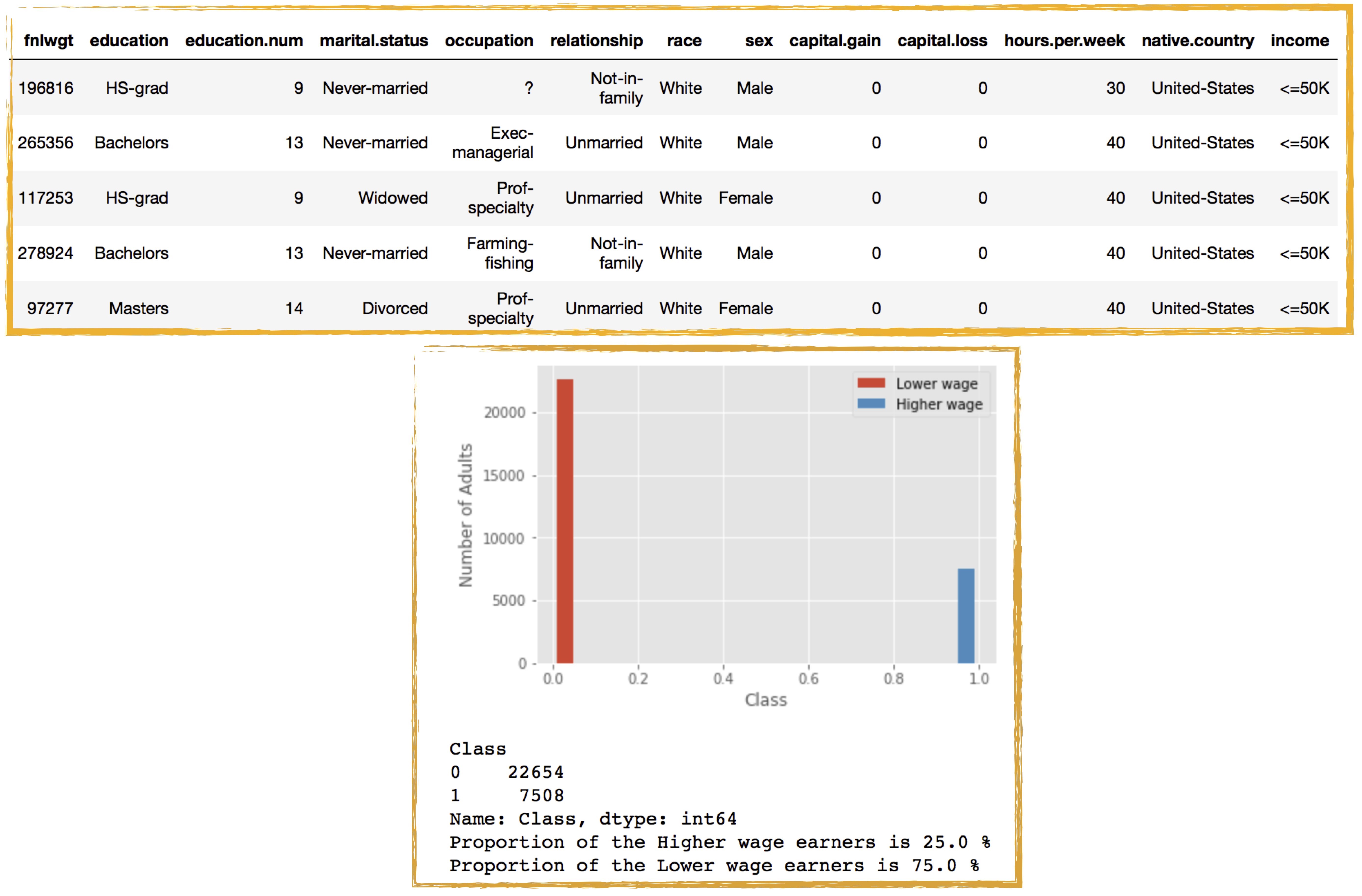
The dataset has both numerical (continuous) and categorical (discrete) features and consists of binary classes, where about 25% of the records in the dataset have a class label of greater than $50,000. There are 14 attributes consisting of eight categorical and six continuous attributes (see text and Table 1 for more details)
3. Impact
This project could have high impact on both industry and research, as it allows datasets such as census, Labour Force Survey, clinical patient record data and any other official admin dataset to be shared more widely and securely for processing and analysis. Our work also yields an exciting avenue to supplement existing datasets, providing a cost-effective way to gather admin and survey data. In scenarios where the real data are scarce, a clear benefit of this work will be the use of synthetic data as a “resource”. Augmentation of real data with synthetic data to build robust statistical, machine and deep-learning models rapidly and cost-effectively to understand and solve real-world problems is one of the overarching goals of this project. A very interesting application of our present work can be to generate synthetic copies of a training dataset with binary classes where the individual classes could correspond to “genuine” and “fake” categories themselves. Although, the present work deals with the generation of dataset(s) with binary classes, its generalisation to multi-class synthetic dataset(s) generation is quite straightforward and might be pursued as a natural extension.
4. GANs operation
When it comes to generating synthetic data, generative models have gathered special attention in the deep-learning community. These are models that can learn to synthesise data that is similar to data used to train the models. The intuition is, if these models can generate new data points that are similar to some of the data points in the training set, the models should have also learnt the underlying structure or representation of the real data. In other words, one of the main problems that generative models are designed to address is the generation of new samples from the same distribution as the training set distribution, that is configure a model that generates synthetic data x obeying a probability distribution psyn(x) that is similar to the (real) data distribution pdata(x).
In recent years, a number of deep-learning methods have captured the interest of the research community with a view to train machines to generate new data. A host of generative models have been developed over the years for a wide spectrum of applications, including generating realistic high-resolution images, text generation and learning interpretable data representations. One such promising approach has been the introduction of generative adversarial networks (GANs) in 2014 by a group of researchers lead by Ian Goodfellow. The basic idea of a GAN is that one trains a network (called a generator) to look for statistical distributions or patterns in a chosen dataset and get it to produce copies of the same. Then a second network (called a discriminator) judges its work, and if it can spot the difference between the originals and the new sample, it sends it back to the generator for further improvements. The first network then tweaks its data and tries to sneak it past the discriminator again. It repeats this until the generator network is creating passable fakes.
In other words, GAN takes a game-theoretic approach when it comes to synthesising new data: it learns to generate data from training distribution through a two-player game. These two networks play a continuous game, where the generator is learning to produce more and more realistic samples, and the discriminator is learning to get better and better at distinguishing generated data from real data. A close analogy will be of a cashier refusing to accept forged currency until the fraudster designs the fake currency identically close to the real currency. This cooperation between the two networks is required for the success of GAN where they both learn at the expense of one another and attain an equilibrium over time; although, it is not always possible for the generator and discriminator to operate at their mathematically optimal values. But, for the sake of completeness, in Appendix A, we derive the optimal values for the operation of the generator and discriminator neural networks originally laid out in From GAN to WGAN. A schematic of a typical GAN architecture comprising a generator and discriminator and outlining its operation is shown in Figure 2.
5. GANs operation - our take
One of the main goals of this project is to generate synthetic data with binary classes, and with this aim in mind we will be focusing our attention on four different flavours of GAN, namely vanilla (normal) GAN, WGAN (Wasserstein GAN), CGAN (conditional GAN) and WCGAN (Wasserstein conditional GAN). It is worth pointing out that when referring to vanilla (normal) GAN architecture, the terminology “GAN” and “vanilla GAN” will be used interchangeably unless stated otherwise. As laid out in Appendix A, the loss function of the vanilla GAN measures the JS divergence between the distributions of pr and pg (for the abbreviations, please refer to Appendix A). Although the vanilla GAN architecture is capable of producing promising synthetic versions of real datasets, the underlying JS divergence metric fails to provide a meaningful value when the pr and pg are disjoint distributions.
One method to further improve the performance of a GAN is to use a better metric of distribution similarity between the two distributions. Wasserstein metric (and thus the name WGAN) is proposed to replace JS divergence because it has a much smoother value space. Wasserstein distance is a measure of the distance between two probability distributions. It is also called Earth Mover’s distance (EM distance) because informally it can be interpreted as moving piles of dirt that follow one probability distribution at a minimum cost to follow the other distribution. The cost is quantified by the amount of dirt moved times the moving distance.
The Wasserstein metric provides criticism of how far the generated dataset is from the real dataset, the “discriminator” network is referred to as the “critic” network in the Wasserstein architecture. In this article we will be comparing the results obtained from both GAN and WGAN, and additionally we will also look into CGAN and WCGAN, where the adversarial network learns to generate samples conditioned (hence the prefix “C”) on the label it takes as input. This will allow us to produce synthetic datasets with more than one class label. Furthermore, adding labels to the data, that is to break it up into categories, has been shown to always improve the performance of GANs and we will thus compare the various GAN architectures against their respective stability as the training progresses.
We based our present analysis on the four different flavours of GANs based on the architectures presented in Create Data from Random Noise with Generative Adversarial Networks. We will generate synthetic versions of our chosen dataset and evaluate the performance of the four different architectures, GAN, CGAN, WGAN and WCGAN. It is worth pointing out that the four different flavours of GANs we have chosen to create copies of synthetic data with is a non-exhaustive list. Not surprisingly, various other training approaches and architectures have been developed to circumvent some of the problems with the original GAN architecture, a non-exhaustive list of some of these architectures is presented in Towards data set augmentation with GANs.
Figure 2: Schematic of a typical GAN architecture comprising of a generator and discriminator
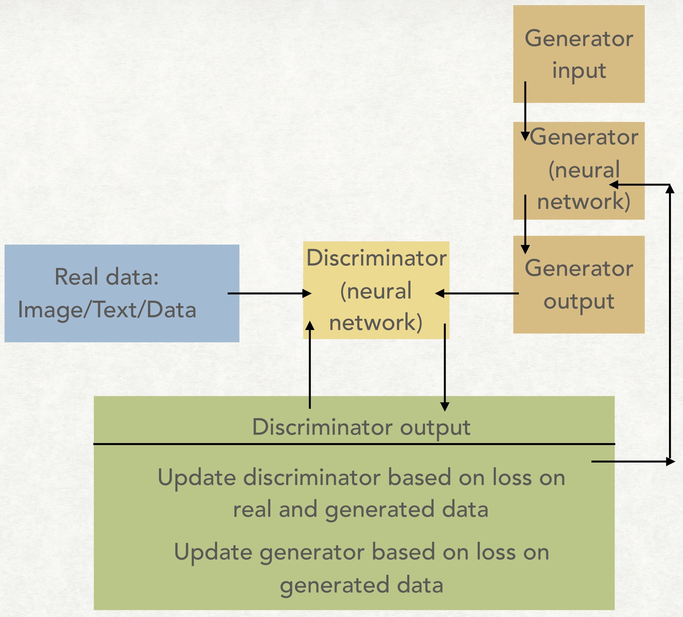
Both the generator and discriminator try to improve their functioning as the training progresses. The GAN pits the generator network against the discriminator network, making use of the cross-entropy loss from the discriminator to train the networks. This is the original, “vanilla” GAN architecture. As outlined in the text, apart from exploring this (vanilla) GAN architecture, we have also investigated three other GAN architectures. The second GAN we have explored introduces class labels to the data in the form of a conditional GAN (CGAN). This GAN has one more variable in the data, the class label. The third GAN uses the Wasserstein distance metric to train the networks (WGAN), and the last one will use the class labels and the Wasserstein distance metric (WCGAN). The cross-entropy loss is a measure of performance of the discriminator in identifying the real and synthetic datasets in GAN and CGAN architectures. The Wasserstein metric instead looks at the distribution of each variable in the real and generated datasets, and determines the distance between the two distributions in WGAN and WCGAN architectures.
About the dataset
The dataset used in this project has 30,162 records and a binomial label indicating a salary of less than $50,000 or greater than $50,000. Of the records in the dataset, 75% have a class label of greater than $50,000. There are 14 attributes consisting of eight categorical and six continuous attributes (Table 1). The employment class describes the type of employer, such as self-employed or federal, and occupation describes the employment type, such as farming, clerical or managerial. Education contains the highest level of education attained, such as high school or doctorate. The relationship attribute has categories such as unmarried or husband, and marital status has categories such as married or separated. The other nominal attributes are country of residence, gender and race. The continuous attributes are age, hours worked per week, education number (numeric representation of the education attribute), capital gain and loss, and a weight attribute that is a demographic score assigned to an individual based on information such as state of residence and type of employment. The continuous variable “fnlwgt” represents final weight, which is the number of units in the target population that the responding unit represents. It is used to weight up the survey results and it is not intrinsic to the population, but an external variable that is dependent on the sample design. However, for the sake of the present analysis we do treat this variable as a “normal” feature and train our GANs on the complete dataset. As we will show later, absence of correlations between this feature and the rest of the features will be evident in the results obtained.
Table 1: Numerical and categorical features of the US adult census dataset. There are six numerical features and eight categorical features in the dataset
| Data variable | Description |
| age (numerical) | Age |
| workclass (categorical) | Type of employment |
| fnlwgt (numerical) | Sampling weight |
| education (categorical) | Level of education |
| education.num (numerical) | Numeric representation of the education attribute |
| marital.status (categorical) | Marital status |
| occupation (categorical) | Occupation |
| relationship (categorical) | Relationship status |
| race (categorical) | Ethnicity |
| sex (categorical) | Gender |
| capital.gain (numerical) | Income from investment sources, apart from wages/salary |
| capital.loss (numerical) | Losses from investment sources, apart from wages/salary |
| hours.per.week (numerical) | Worked hours per week |
| native.country (categorical) | Native country |
Numerical features
Our aim is to train the different models of GANs in order to synthesise data belonging to the two different classes of the US adult census dataset. Because of the known problems in GANs in generating discrete (categorical) data features, we will first focus on training our GAN architectures by only considering the numerical (continuous) features present in the dataset. We will then briefly look into ways of representing categorical (discrete) features as continuous features and using this transformed representation for training our GANs. For our present work, we follow the steps laid out in Figure 3 to generate synthetic copies of the adult census dataset using the four different variations of GANs. The first step involves scaling the data. As we do not want any one specific feature to dominate the training procedure of our neural network we rescale all the feature values between 0 and 1. We then use this transformed dataset to train our four different GAN models and finally perform a range of data quality checks to test the performance of our synthetic data models. A pair plot of the rescaled dataset (containing only the numerical features) is shown in Figure 4.
Table 2: Hyperparameters used in the four different flavours of GANs.
| Hyperparameter | Value |
| Batch size | 128 |
| Number of steps to pre-train the critic before starting adversarial training | 100 |
| Number of training steps | 5000 |
| Learning rate | 5e-5 |
| Hidden layers | 3 |
| Activation function | ReLU (Rectified Linear Unit) |
The batch size defines the number of training samples that will be propagated through our deep neural networks. ReLU is one of the most commonly used activation functions in the neural networks and deep learning that is responsible for introducing nonlinearity to models to learn nontrivial structures and patterns in the datasets.
Training GANs: We split the adult census dataset into training and testing sets. Since our original data are comprised of unbalanced classes we split the data in a stratified fashion to ensure that the split data are proportionally representing the values of Class column, that is, the two wage classes categories are present both in train and test data proportionally. The entire training procedure was conducted on a laptop with standard specifications (2.2 GHz Intel Core i7) and use of GPU was not required.
Figure 3: A schematic showing the different steps involved in our synthetic data generation framework
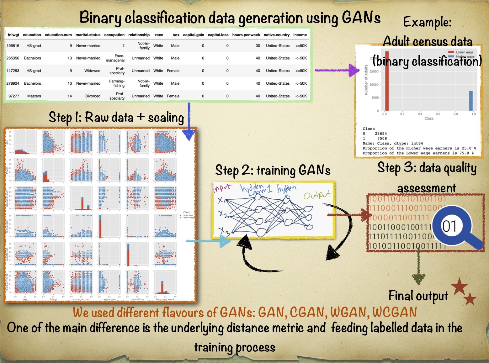
The first step involves scaling the data (rescaling all the feature values between 0 and 1). We then use this rescaled dataset to train our four different GAN models for a number of training steps. The data quality checks are performed after synthetic copies of the datasets are obtained using the four different flavours of GANs
Our GAN architectures were implemented in Python using the Keras library and a TensorFlow back-end as originally developed in the guiding work for our project. The generator and discriminator in all the four different flavours of GANs are deep neural networks and their layered architectures as used in our framework are shown in Figure 5. Both the discriminator and generator have three hidden layers with the generator having n input and n output units and the discriminator with n input units and one output unit (where n is the number of features in the input dataset).
As shown in Figure 5, the hidden layers in our networks are densely connected layers where the neurons in densely connected layers are connected to every input and output of the layer, allowing the network to learn its own relationships among the features including any potential (non) linear correlations amongst the features. The performance of neural networks depends heavily on the choice of hyperparameters in the training process: choice of architecture, activation functions and learning rate, to mention just a few. GANs double these challenges because of the involvement of two competing neural networks. For our GAN architectures we will focus on the set of hyperparameters shown in Table 2. It is worth noting that we have not optimised the hyperparameters tabulated in Table 2 and we have arrived at these numbers following a trial and error scheme. However, tuning of these hyperparameters remains an interesting avenue to be explored further but was not the focus of our present work.
Synthetic data outputs from GANs: We train our four different GAN architectures on the training dataset and for the sake of visual comparison we plot two numerical features (age and hours per week) of the generated synthetic datasets for increasing the number of training steps, as shown in Figure 6. Looking at Figure 6, for the set of hyperparameters we have chosen (Table 2), (vanilla) GAN is particularly unstable while the best performance is achieved using WCGAN architecture. It is also worth mentioning that under GAN and WGAN the class label is not present and so the resulting outputs do not have a class distinction. Since WCGAN architecture is shown to produce the most promising results for our choice of parameters, we will therefore exclusively focus on the synthetically generated data under the WCGAN architecture.
Figure 4: A pair plot of the numerical features of the census dataset shown for the two different wage classes
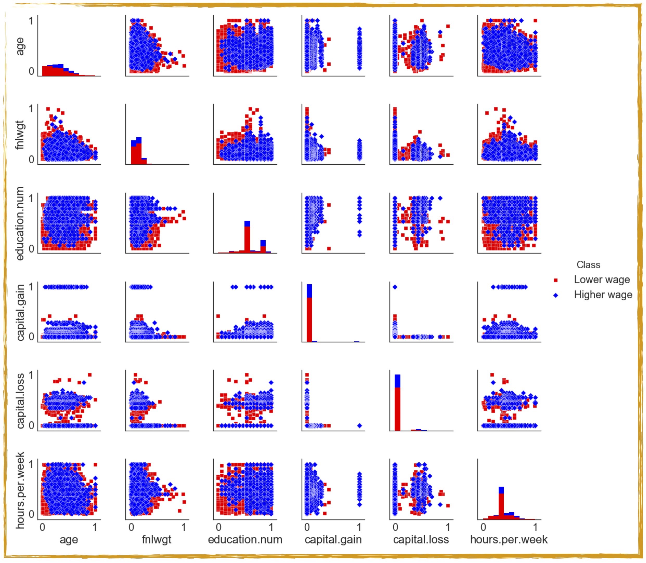
The plot illustrates the pairwise relationships between the numerical features of our dataset. The dataset (with six numerical features) has been transformed to a grid of axes such that each numerical feature in the dataset will be shared in the y-axis across a single row and in the x-axis across a single column. The diagonal axes show the univariate distribution of the data for the variable in that column.
Apart from producing synthetic data similar to real data, our WCGAN model also gets trained to output the “outliers” present in the original dataset. One could also perform a feature-wise comparison of the data generated by the WCGAN and the real dataset. In Figure 7 we show such a comparison by producing pair plots for both real and synthetic datasets. It is evident from Figure 7 that output of our WCGAN models is promising but it is not perfect. For instance, we observe that the model is capable of generating (visually) similar features to the (real) features when the corresponding distribution space is uniform in the latent space and is not too discretised. For example, looking at the diagonal components of real and synthetic scatter matrices in Figure 7 one could easily observe that the WCGAN model produces (visually) similar synthetic copies for features such as ”age”, “fnlgwt”, “hours.per.week” but not so similar synthetic copies for features such as “education.num”, “capital.gain” and “capital.loss”. It is worth stressing that synthetic data generation using GANs involves approximating the true (data) distribution with some variation – the error tolerance between the actual and synthetic data distribution depends on the application at hand. We will next focus on assessing the quality of the generated data.
Synthetic data quality assessment: We will employ a number of methods to assess the data quality of our synthetic data models. As a first metric to evaluate the quality of the synthetically generated data, we compute the pairwise cross-correlation on the generated dataset and for the sake of comparison also evaluate the pairwise cross-correlation on the training dataset as shown in Figure 8. To assess the discrepancy between the synthetic and real datasets we evaluate the cross-correlation matrix difference, which is obtained by the subtraction of the cross-correlation matrix of the real dataset and the generated dataset. If the two datasets are well matched this will be close to zero for the whole matrix and as can be seen from Figure 8 there is evidently a room for improvement.
Figure 5: The discriminator and generator neural network layered architectures as used in all the four flavours of GANs for synthesising numerical features of the US adult census dataset
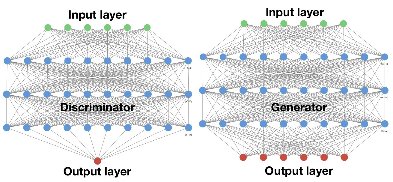
Both the discriminator and generator have three hidden layers with the generator having six input and six output units and the discriminator with six input units and one output unit.
To further ensure that our WCGAN model has reached a level of stability over training time, we also evaluate the critic loss as the difference between the loss functions of the discriminator and generator. The critic loss function and the correlation matrices are shown in Figure 8. It is clear that compared with traditional GAN training, W(C)GAN training is more stable, which is reflected in the behaviour of its respective loss function.
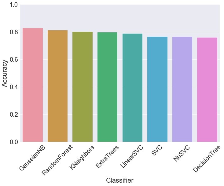
We started the synthetic data generation problem by training various GAN architectures on a dataset with different classes. As another metric to assess the data quality of WCGAN output, we train a set of classifiers on the synthetically generated dataset and subsequently test their performance on an (unseen) real test dataset as shown in Figure 9. While testing the performance accuracy of our chosen set of classifiers we ensured that both the classes present in our dataset were assigned balanced weights in the training procedure. This metric of accessing the data quality is independent of the underlying data distribution and can be seen purely in terms of evaluating the usage of synthetically generated data as a resource for data science applications. Specifically, one of the most appealing applications of synthetic data generation is data augmentation and this metric could be a quick way of assessing if synthetic data has a high quality to replace or supplement the real data. Similar average classification accuracy was obtained on training the chosen set of classifiers on the real data and testing their performance on synthetic datasets.
To ensure that our GAN architectures are learning the original data distribution and not simply memorising and reproducing the training data, we follow a recipe introduced in Airline Passenger Name Record Generation using Generative Adversarial Networks. We calculate the Euclidean distances between each generated point and its nearest neighbour in the (real) training and test datasets. We then compare the distributions of distances using the Mann-Whitney U test, Wilcoxon Test and Kruskal-Wallis H-test to determine if they differ. These are nonparametric statistical significance tests for determining whether two independent samples were drawn from a population with the same distribution. High p-value for these tests would imply that the two samples were drawn from the same population.
On running these tests, we found that the resulting p-values for each of these tests was higher than the significance level (0.05), and we thus fail to reject the null hypothesis that the two distributions were different. This can be interpreted as our generative model architecture (WCGAN in this case) not simply memorising the training set but rather learning its distribution. Histogram of the distances between the generated samples and the nearest neighbours in the training and test sets is shown in Figure 10. The Pearson correlation coefficient shown in Figure 10 measures the linear relationship between the two distributions. Like other correlation coefficients, this one varies between negative 1 and positive 1 with 0 implying no correlation. Correlations of negative 1 and positive 1 imply an exact linear relationship. Positive correlations imply that as x increases, so does y. Negative correlations imply that as x increases, y decreases. The p-value roughly indicates the probability of an uncorrelated system producing datasets that have a Pearson correlation at least as extreme as the one computed from these datasets.
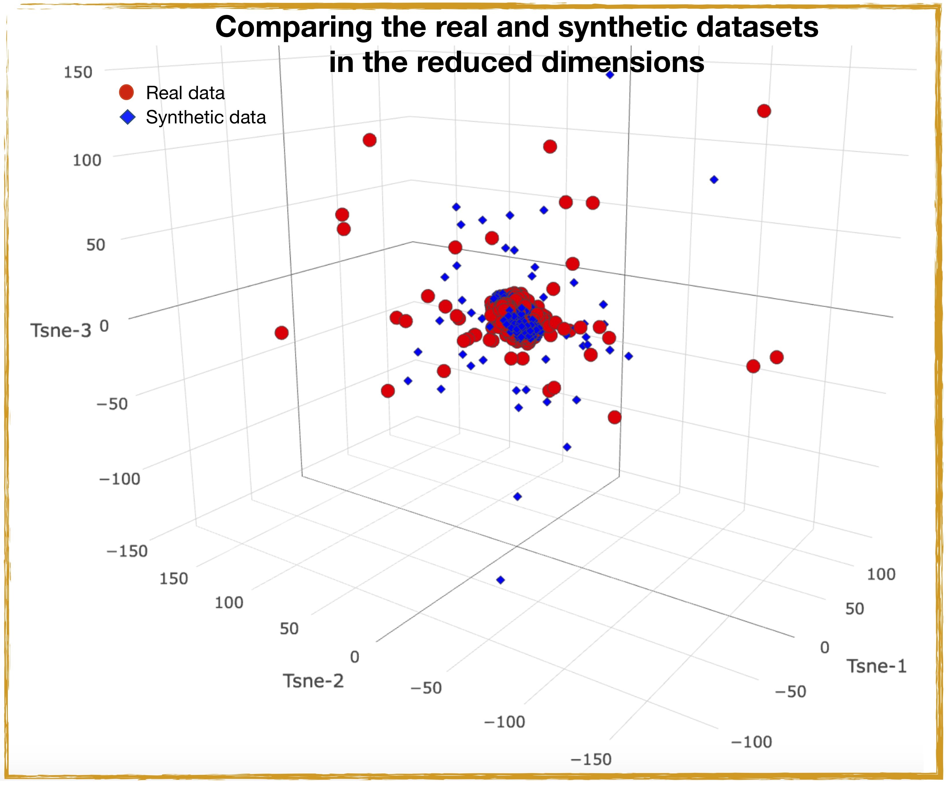
Since the generated dataset and real datasets are multidimensional, to (visually) compare the two datasets we apply the t-Distributed Stochastic Neighbor Embedding (t-SNE) on our real and synthetic datasets. This technique allows for dimensionality reduction that is particularly well suited for the visualisation of high-dimensional datasets.
Figure 6: Comparing the performance of different GAN architectures as a function of number of training steps
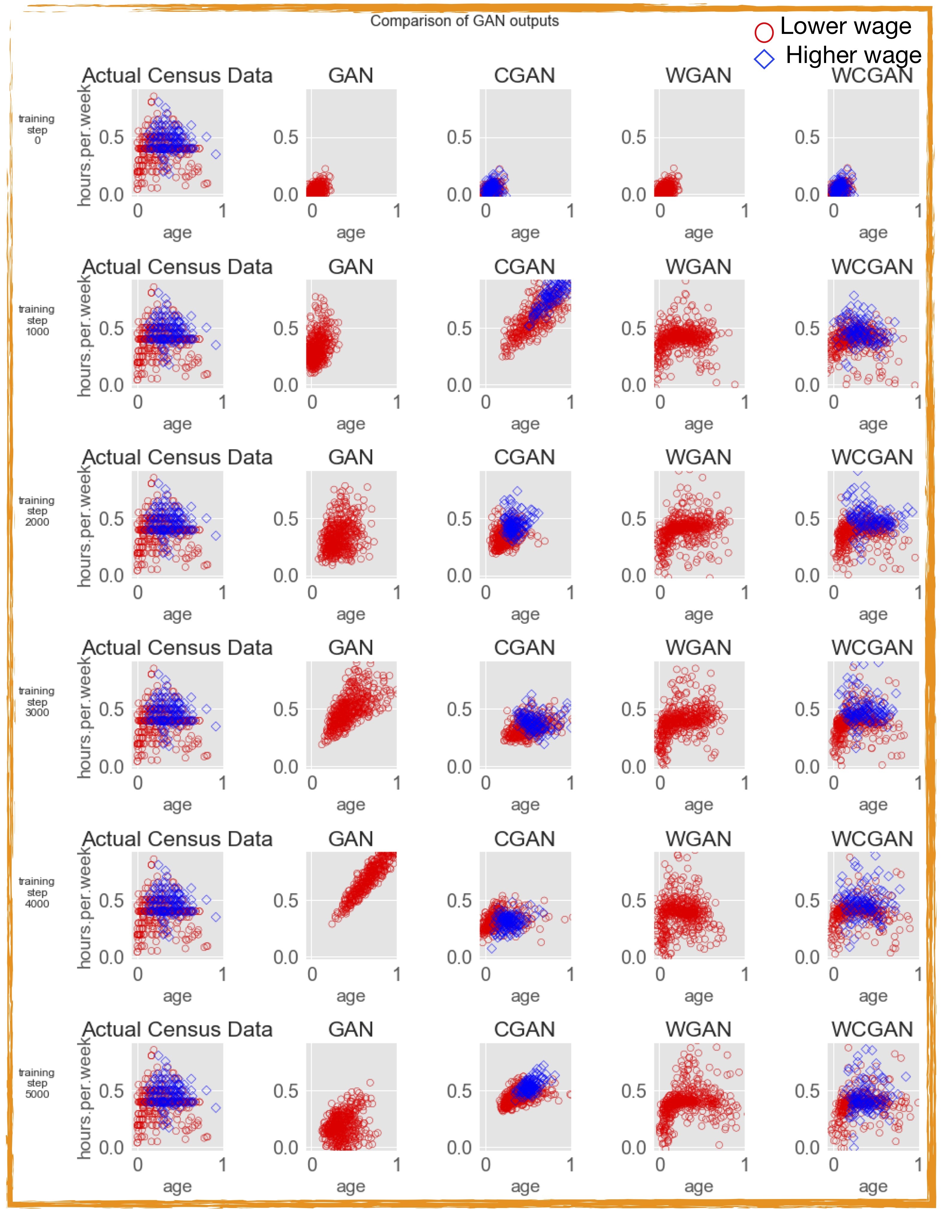
Out of the four different flavours of GANs, WCGAN seem to perform most stably while the (vanilla) GAN is the least stable as the training progresses. At step 0, all the generated data shows the normal distribution of the random input fed to the generator of all four GANs
The t-SNE algorithm models each high-dimensional object by a two- or three-dimensional point in such a way that similar objects are modelled by nearby points and dissimilar objects are modelled by distant points with high probability. Comparison of the t-SNE real and the synthetic datasets in the three-dimensional space is shown in Figure 11. Again, Figure 11 shows that in the t-SNE manifold, most of the data points in both the datasets are centred close to each other with a few outliers extending beyond the main blob, signalling the similarity between the real and synthetic datasets.
Figure 7: Pairwise comparison of the numerical features of the real and synthetic (WCGAN) datasets. The synthetic data shown here are obtained by training WCGAN architecture for 5,000 steps
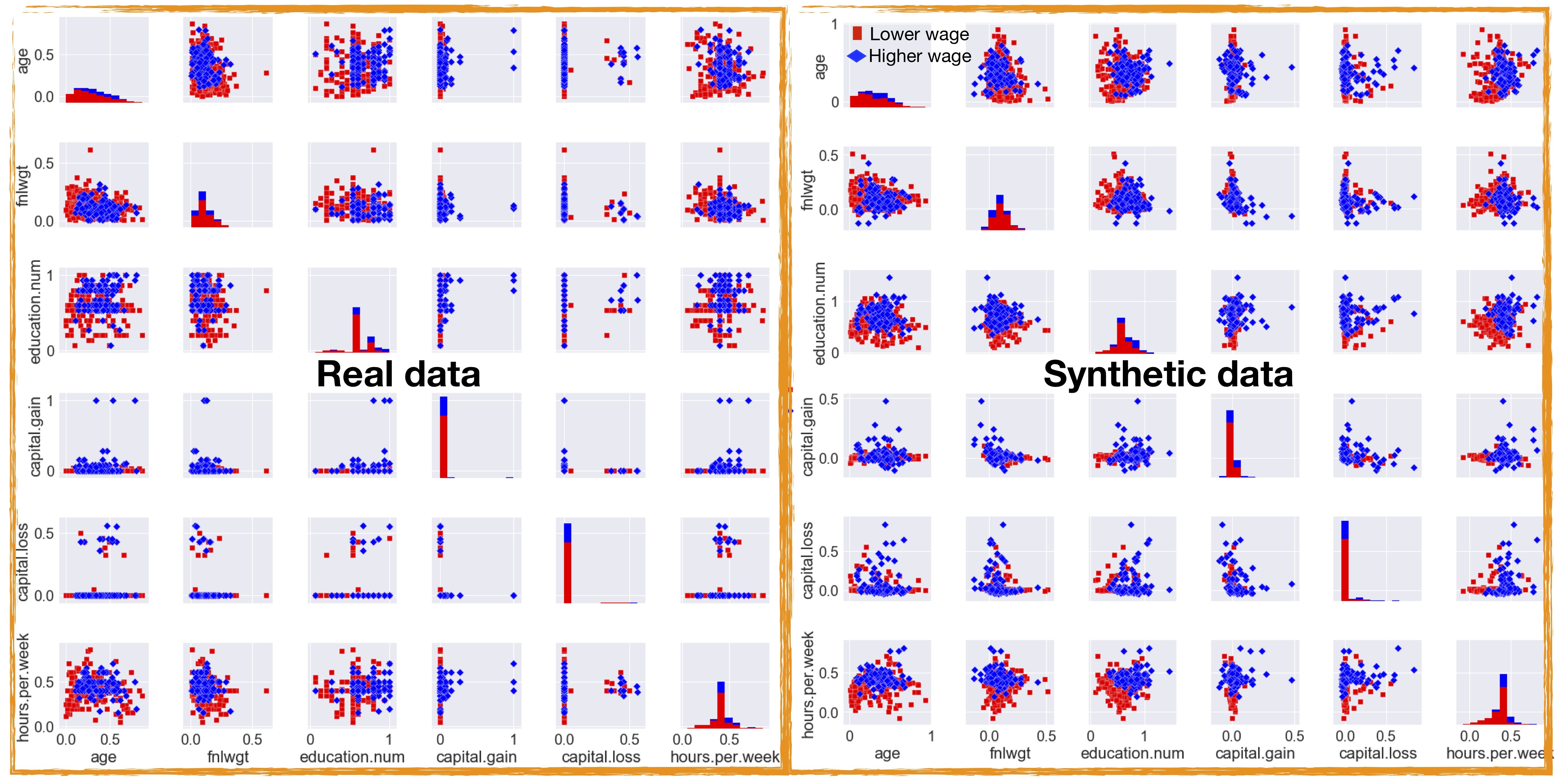
Figure 8: Pairwise correlation matrix evaluated using the real and synthetically generated datasets
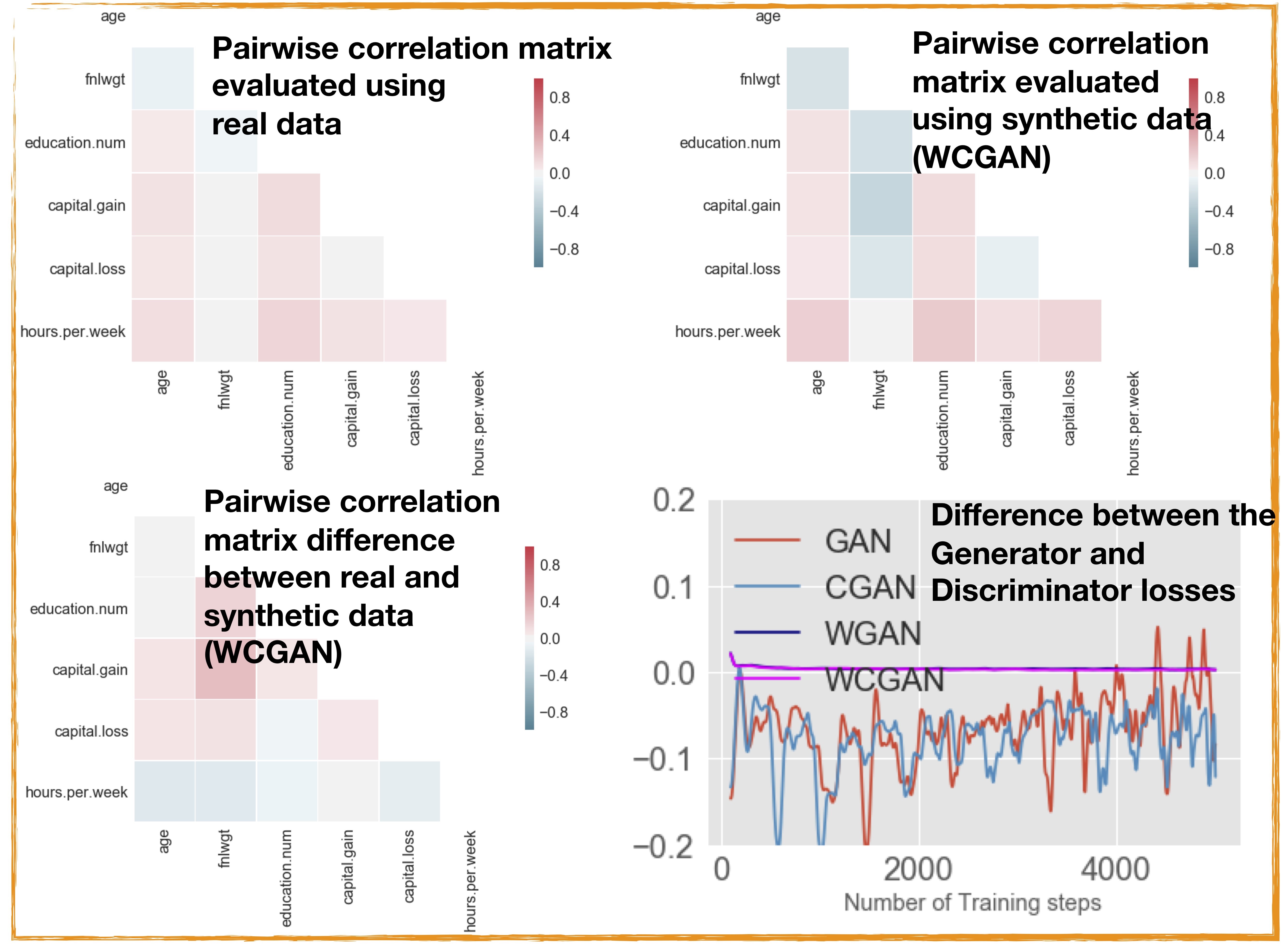
Also shown is the critic loss functions shown here as a function of number of training steps for different GAN architectures. From the loss function of the respective four GANs it is evident that compared with traditional GAN training, W(C)GAN training is more stable, which is reflected in the relatively smoother transitioning of its respective loss function to zero. The loss functions of WGAN and WCGAN are almost indistinguishable as the training progresses.
Figure 9: Average classification accuracy of the classifiers trained on synthetic data and tested on test dataset is 76.12%
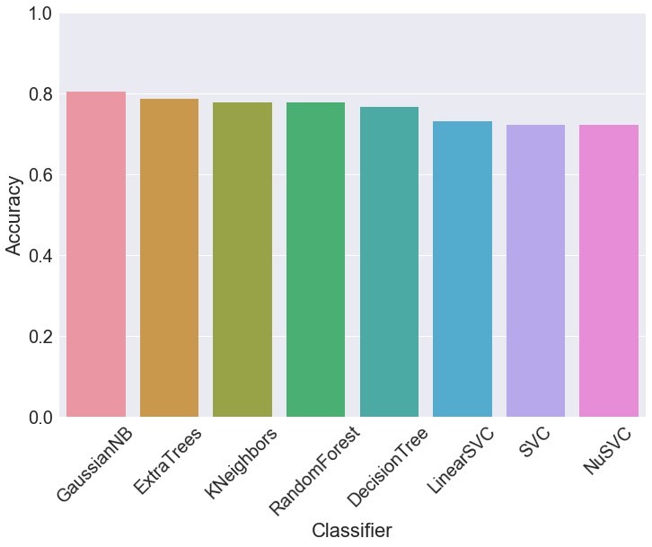
On the other hand, average classification accuracy of the classifiers trained on real data and tested on synthetic dataset (not shown above) resulted in an accuracy score of 78.25%. While testing the performance accuracy of our chosen set of classifiers we ensured that both the classes present in our datasets (both real and synthetic datasets) were assigned balanced weights in the training procedure.
Categorical features
As we mentioned before, GANs are notorious for generating discrete data. GANs work by training a generator network that outputs synthetic data, then running a discriminator network on the synthetic data. The gradient of the output of the discriminator network with respect to the synthetic data tells us how to slightly change the synthetic data to make it more realistic. One can make slight changes to the synthetic data only if it is based on continuous numbers. If it is based on discrete numbers, there is no way to make a slight change. The adult census data are a mixture of discrete and continuous features. To deal with the categorical features in our dataset we use a relatively simple strategy recently outlined. Under this approach, discrete columns are encoded into numerical [0,1] columns using the following method. Discrete values are first sorted in descending order based on their proportion in the dataset. Then, the [0,1] interval is split into sections [ac,bc] based on the proportion of each category c. To convert a discrete value to a numerical one, we replace it with a value sampled from a Gaussian distribution centred at the midpoint of [ac,bc] and with standard deviation σ = (bc − ac)/6.
One could again evaluate the performance of our synthetic data architecture after applying the these transformations to the categorical variables and compare each of the features of the generated dataset against the real dataset respectively. But due to the increase in the number of features, we choose not to show a feature-wise comparison of the real and the synthetic datasets. Instead, we quantify the quality of our synthetically generated dataset by training a set of classifiers on the synthetically generated dataset and testing their performance on an (unseen) test real dataset with the resulting plot shown in Figure 12. As done with the numerical features, while testing the performance accuracy of our chosen set of classifiers we ensured that both the classes present in our dataset were assigned balanced weights in the training procedure.
Figure 10: Histogram of the distances between the generated samples and the nearest neighbours in the training and test sets. Also shown is a joint plot of the two distance distributions
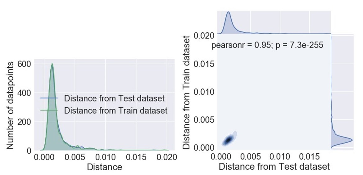
Figure 11: T-sne transformed real and synthetic datasets in the reduced t-SNE transformed space
The resulting average classification accuracy of the classifiers (trained on synthetic data) and tested on test dataset was found to be close to 80%. This result is again a good indicator of our framework generating good-quality data fit for data augmentation tasks. Strictly speaking, turning of discrete values into continuous variables should be done in conjunction with the final weight (fnlgwt) feature to correct to the real population. But we leave this for a future investigation.
The problem of synthetic categorical data generation using the GAN framework is a difficult one and we are currently pursuing more sophisticated methods including word embeddings and embedding layers in a deep neural network to convert one hot encoded variables into vector representation to get better results. We plan to explore a deep neural network outlined in a recent work on Entity Embeddings of Categorical Variables, which has shown promising results.
Figure 12: Average classification accuracy of the classifiers (trained on synthetic data) and tested on test dataset is 78.8%. The categorical variables in the dataset have been transformed according to the strategy outlined in the text
6. Problems in GANs
Although generative adversarial networks (GANs) can easily qualify as one of the most advanced deep-learning architectures, they do suffer from some fundamental problems outlined in various places [see From GAN to WGAN, and GAN? – Why it is so hard to train Generative Adversarial Networks!]. The following are some of the known problems with GAN architectures:
- GANs are hard to train and the process can be slow and unstable. The discriminator and the generator models are trained simultaneously to find a Nash equilibrium to a two-player non-cooperative game. However, each model updates its cost independently and this cannot guarantee a convergence.
- GANs also suffer with the problem of vanishing gradient. If the discriminator behaves badly, the generator does not have accurate feedback and the loss function cannot represent the reality. If the discriminator does a great job, the gradient of the loss function drops down to close to zero and the learning can become very slow.
- During the training process, the generator may collapse to a setting where it always produces the same outputs. This is a common failure case for GANs, commonly referred to as mode collapse. In such a scenario, the generator only learns a small distribution of the real-world data distribution and gets stuck in a small subspace. In the exploratory phases of this project, while testing our GANs models on other toy datasets, we found that the problem of mode collapse can be circumvented by using the WGAN architecture as known in GAN – Why it is so hard to train Generative Adversarial Networks!.
- GANs do not come with a good objective function; this makes it very difficult to assess the training progress and compare the performance of multiple models.
- Generating categorical data is a particularly difficult problem for GANs.
7. Limitations of synthetic data
Synthetic data generation methods score very high on cost-effectiveness, privacy, enhanced security and data augmentation to name a few. However, synthetic data generation models do come with their own limitations. While synthetic data can mimic many properties of real data, by their very design the synthetic data generation models we have discussed do not recreate the original data exactly. At the same time, any analysis on synthetic data needs to be verified on the real dataset. Synthetic data generative models look for common trends in the real data when creating synthetic data, but may not capture any anomalies present in the real data. In some instances, this may not be a critical issue. However, in other scenarios, this will severely limit the capabilities of the model and negatively impact the output accuracy.
Not surprisingly, the quality of synthetic data is highly dependent on the quality of the model that created it. The generative models we have focused our attention on can be excellent at approximating the data distribution of the original datasets, uncovering the underlying patterns in the datasets, recognising statistical regularities in datasets but at the same time they can also be susceptible to statistical noise, such as adversarial perturbations. Adversarial perturbations can cause the model or network to completely misclassify data and in turn, create highly inaccurate outputs.
Another challenge presented by using synthetic data is the need for a verification procedure to test and compare the real and synthetic data outputs. This is to ensure the model(s) has been properly trained and is not generating the desired outputs due to any assumptions that were built into the synthetic data. The validation is a way of making sure that the assumptions that were built into the synthetic data are not driving the results. Due to the complexity and varied nature of datasets available to us today, the best one could hope for is the possibility to generate customised synthetic datasets in the future while not attempting to design a universal synthetic data generation tool.
8. Conclusions
In this project we embarked on the problem of generating synthetic data with a few different flavours of generative adversarial networks (GANs). Although the end results have been promising we want to point out that we have barely scratched the surface of the synthetic data generation problem with these methods. To further improve the quality of the results, we could try a number of improvements, including training the models for an increased number of steps, increasing the number of hidden layers in the network, and, of course, by further tuning the hyper parameters for the various GAN architectures. Furthermore, to improve the quality of GAN architecture, one could try various other approaches including feature matching, minibatch discrimination, historical averaging, one-sided label smoothing, virtual batch normalisation, and adding noise.
Synthetic data are a powerful tool when the required data are limited or there are concerns to safely share it with the concerned parties. When data privacy is a requirement and the generated data are prone to attacks from sophisticated attackers with lots of computational power, we recommend the use of GANs possibly in conjunction with privacy-preserving mechanisms such as differential privacy.
We have used four different GAN architectures to generate synthetic copies of the US adult census dataset with binary classes.
Different GAN architectures differ in the quality of the generated synthetic data, where one specific architecture Wasserstein GAN (WGAN) is shown to give the best performance avoiding some of the known issues with training normal GANs such as mode collapse.
The quantitative results from our experiments on synthetic data generation with several methods suggest that our framework is capable of producing high-quality synthetic samples as the Pearson correlation structure of the real data was closely reflected by the correlation structure of the synthetic data, indicating relations between the variables in the original data are preserved in the synthetic data.
One of the most appealing applications of synthetic data generation is data augmentation and to ensure if our generated synthetic data has a high quality to replace or supplement the real data we trained a range of machine-learning models on synthetic data and tested their performance on real data whilst obtaining an average accuracy close to 80%.
We show that synthetic data generative methods such as GANs are learning the true data distribution of the training dataset and are capable of generating new data points from this distribution with some variations and are not merely reproducing the old (training) data the model has been trained on. We have confirmed this finding using a range of nonparametric statistical significance tests.
GANs are an active area of research and new variants of GANs are coming up frequently. For instance, the Cram´er Generative Adversarial Network has been shown to perform significantly better than the related Wasserstein GAN architecture. We could integrate methods that make use of semi-supervised learning, which can be a promising approach when the training dataset is limited (see Improved Techniques for Training GANs).
Synthetic data generation methods score very high on cost-effectiveness, privacy, enhanced security and data augmentation to name a few. However, synthetic data generation models do come with their own limitations. While synthetic data can mimic many properties of real data, by their very design the synthetic data generation models we have investigated do not recreate the original data exactly. At the same time, any analysis on synthetic data needs to be verified on the real dataset.
The quality of synthetic data is highly dependent on the quality of the model that created it. The generative models we have focused our attention on can be excellent at approximating the data distribution of the original datasets, uncovering the underlying patterns in the datasets, recognising statistical regularities in datasets but at the same time, they can also be susceptible to statistical noise.
Due to the complexity and varied nature of datasets available to us today, our findings suggest that the best one could hope for is the possibility to generate customised synthetic datasets in the future while not attempting to design a universal synthetic data generation tool. Our findings in this work suggest that even in the situations where it is necessary to generate synthetic data it should always be mixed with reality to make informed decisions.
Overall, the synthetic data generation using GANs is a research-intensive field and we are hopeful that future work on the project and subsequent improvements on the architecture could lead to the generation of high-quality data useful for a variety of applications.
Our next steps will be to further improve the operation of our synthetic data generation models through hyperparameter optimisation, explore other variants of GANs, explore GANs for discrete data and perform a more quantitative analysis on the quality of the generated data. Eventually, we are working towards making our synthetic data generation framework fit for purpose to produce good-quality datasets for real-world applications, including census and clinical data.
9. Appendix A: GANs operation – optimal values of generator and discriminator
The generator forms a crucial component in the functioning of GAN and performs a mapping ˆx =G(z), where z is some random noise. Its goal is to produce samples, x, from the distribution of the training data p(x) as outlined here. The discriminator forms the second competing process in a GAN. Its goal is to look at sample data (that could be real or synthetic from the generator), and determine if it is real (D(x) closer to 1) or synthetic (D(x) closer to 0). D(x) can be interpreted as the probability that the sample data are drawn from a real (training) dataset. To succeed in the game, the generator must make samples that are indistinguishable to the discriminator. Under such a perfect Nash equilibrium, the optimal value of D(x) = 1/2, where generator is a perfect generative model sampling from the real data.
One of the chief metrics when it comes to evaluating the performance of GANs depends on quantifying the similarity between two probability distributions. When it comes to discriminating two probability distributions, the following metrics are often used:
Kullback-Leibler (KL) divergence
This measures the divergence between an observed probability distribution p(x) and expected probability distribution q(x). KL divergence is defined as follows:
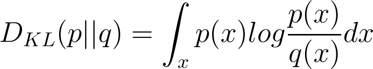 |
(1) |
It is noticeable according to the formula that KL divergence is asymmetric. One problem with this metric is it fails to capture the divergence between the two distributions in cases, where p(x) is close to zero but q(x) is significantly non-zero, the q’s effect is disregarded.
Jensen-Shannon (JS) divergence
It is another measure of similarity between two probability distributions, it is symmetric with respect to the two distributions and is bounded between 0 and 1.
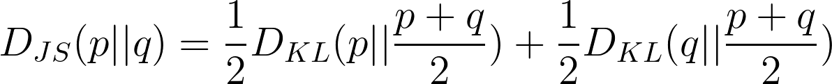 |
(2) |
GANs use the above as its loss function.
The generator G and the discriminator (critic) model D compete against each other during the training process, where G is trying hard to trick the discriminator, while D is trying hard not to be cheated. This interesting zero-sum game between two models motivates both to improve their functionalities. Before explicitly identifying the loss function in a GAN, let us first illustrate some of the notations involved.
| pz ∼ (Uniform) data distribution over noise input z
pg ∼ The generator’s distribution over data x pr ∼ Data distribution over real sample x |
(3) |
On the other hand, the discriminator’s goal is to maximise:
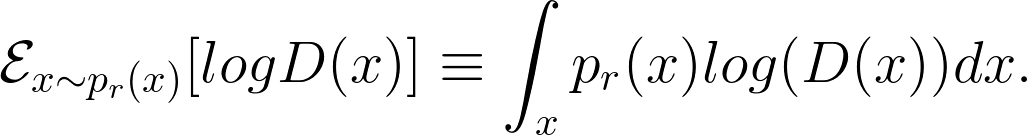 |
(4) |
Meanwhile, given a fake sample G(z),z ∼ pz(z), the discriminator is expected to output a probability, D(G(z)) close to zero by maximising
 |
(5) |
At the same time, the generator is trained to increase the chances of D producing a high probability for a fake example, and thus to minimise
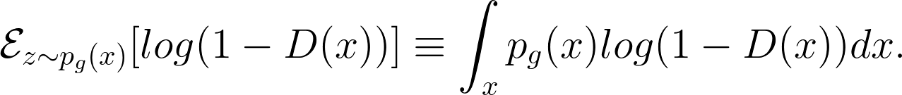 |
(6) |
When combining the both aspects together, D and G are playing a minimax game in which we should optimise the following loss function:
 |
(7) |
After arriving at the above well-defined loss function, it is a matter of computing a simple first order derivative to arrive at the best value of the discriminator
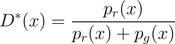 |
(8) |
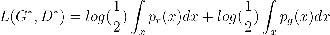
Once the generator is trained to its optimal value, pg ≈ pr and the optimal value of the discriminator is set to D∗(x) → 1/2. The global value of the loss function when G,D are at their optimal values can be easily evaluated as follows:

|
(9) |
In the case of above optimal values, the JS divergence between pr and pg can be computed as:
 |
(10) |
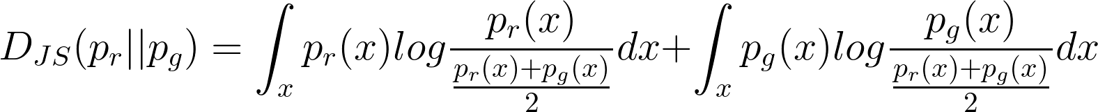 |
(11) |
 |
(12) |
| (13) | |
| |
(14) |
It can be seen from above that under the JS divergence the loss function of GANs quantifies the similarity between the generative and the real sample distributions when the discriminator is optimal. The best generator is G∗ that replicates the real data distribution and leads to the minimum value of L(G∗,D∗) = −2log(2).
10. Authors
11. References
Ian J Goodfellow, Jean Pouget-Abadie, Mehdi Mirza, Bing Xu, David Warde-Farley, Sherjil Ozair, Aaron Courville, Yoshua Bengio, Generative Adversarial Nets
Prakash Pandey, Deep Generative Models
Christies.com, Is artificial intelligence set to become art’s next medium?
AI Wiki, A Beginner’s Guide to Generative Adversarial Networks (GANs)
UC Irvine Machine Learning Repository, Adult census dataset
UC Irvine Machine Learning Repository, Breast Cancer Wisconsin (Diagnostic) dataset
Anonymized credit card transactions labeled as fraudulent or genuine, Credit card fraud detection dataset
Li´lLog, From GAN to WGAN
Fei-Fei Li, Justin Johnson, Serena Yeung (2017 Lecture), Generative Models as covered in CS231n: Convolutional Neural Networks for Visual Recognition
Shakir Mohamed, Balaji Lakshminarayanan, Learning in Implicit Generative Models
Martin Arjovsky, Soumith Chintala, and L´eon Bottou, Wasserstein GAN
Mehdi Mirza, Simon Osindero, Conditional Generative Adversarial Nets
Cody Nash, Create Data from Random Noise with Generative Adversarial Networks
Pedro Ferreira, Towards data set augmentation with GANs
reddit, Generative Adversarial Networks for Text
Alejandro Mottini, Alix Lh´eritier, Rodrigo Acuna-Agost, Airline Passenger Name Record Generation using Generative Adversarial Networks
Laurens van der Maaten, Geoffrey Hinton, Visualizing Data using t-SNE
One hot encoding The way one hot encoding works is, it takes a column which has categorical data, which has been lab
Yonatan Hadar, Using categorical data in machine learning with python: from dummy variables to Deep category embedding and Cat2vec -Part 2
Cheng Guo, Felix Berkhahn, Entity Embeddings of Categorical Variables
Jonathan Hui, GAN? – Why it is so hard to train Generative Adversarial Networks!
Marcelo Benedetti, The advantages and limitations of synthetic data
Omid Poursaeedi, Isay Katsman, Bicheng Gao, Serge Belongie Generative Adversarial Perturbations
Marc G Bellemare and others, The Cramer Distance as a Solution to Biased Wasserstein