Discovering emerging important terminology in large text datasets using pyGrams: a comparison between net growth and e-score methods

In pyGrams: An open source tool to discover emerging terminology in large text datasets, we discussed how pyGrams could be used to extract important terminology from free text. Here, we expand on the analysis of term usage over time for data that have a temporal component. This type of work in data science is called time series analysis.
The objective of this work is to identify important words, “the main terminology”, in large text datasets and track their use over time. This will help an analyst discover emerging or fading terminology or, in the case of the patents data, emerging technology. A new method, called net growth, has also been developed and tested.
For the reader’s convenience, here we define several concepts adopted in this report. First, we refer to data with a temporal component as a time series. Secondly, we define emergence as becoming known or growing over time. Here, for the frequency of terminology, an emerging term is therefore one whose frequency increases over time within a user-defined period. As a result, an emergence score is used in this report to quantify emerging terminology, whereby the larger the emergence score, the faster the terminology grows.
In pyGrams: An open source tool to discover emerging terminology in large text datasets, we showed how our Python tool, pyGrams, could be used to extract important terminology from patents built around a term frequency–inverse document frequency (tf–idf) approach. In this report, we focus primarily on how pyGrams can be used to analyse terms through time using the time stamps in document metadata.
For patents, identifying an emerging technology early is important. Early identification can inform decisions by policymakers or other decision-makers prior to large-scale take-up of technologies or components or their adoption into manufacturing processes. This early identification can allow organisations and individuals to allocate suitable resources to address future technological trends and requirements more efficiently. An example of this would be cheap access to unmanned aerial vehicles (UAVs) to the general public, which meant the UK Civil Aviation Authority (CAA) had to create a new set of guidance and regulations for users.
In the future, self-driving vehicles are likely to require organisations such as the Driver and Vehicle Licensing Agency (DVLA) to update their own policies. In addition, early identification of emerging technologies such as climate change-mitigation technologies may be supported or encouraged through economic incentives.
The work developed for pyGrams, although created with patent datasets in mind, is not restricted in its use only to patents. This tool can be – and in some instances already has been – used to help identify emerging terminology in other fields. For academic journals, the early identification of new research methods may help countries and universities develop expertise in certain research topics sooner to meet increasing future demand. When used on job adverts, the tool can be used for an understanding of the emerging skills required for specific roles such as Data Scientist. Such findings mean that companies can tailor their recruitment to improve their talent pool, and job seekers can build the right skills.
Table of contents
1. Methods
To identify the emergent terms of a given text dataset, pyGrams uses the following approach:
- embed the text corpus into a term frequency–inverse document frequency (tf–idf) matrix*
- generate a dictionary of n number of candidate terms from the corpus*
- generate time series data for the selected terms from the tf–idf matrix*
- smooth the time series
- analyse the resulting smoothed time series data for emerging or declining terms
*The processes behind steps one, two and three are explained in more detail in pyGrams: An open source tool to discover emerging terminology in large text datasets. This report focuses on steps four and five.
Time series smoothing
During initial experiments, it became apparent that the patent dataset was prone to volatility and noise. This volatility and noise would make time series analysis challenging. It is also likely to affect the quality of the subsequent emergence score calculations and trend forecasts. Therefore, to remove the noise, we smoothed the time series. We used two smoothing methods: the state-space model using the Kalman filter and the Savitzky–Golay filter.
The Kalman filter is ideal for solving linear problems and for dynamic systems where you need to estimate what the system will do next. The Savitzky–Golay filter fits a polynomial in a window of points around each sample point, using least squares fitting. The major benefit of Savitzky–Golay is that it helps preserve the area, position and width of peaks in the original data. The Kalman filter is a more accurate method, but it is slow to use on large datasets, whereas the Savitzky–Golay filter is a faster alternative.
In addition, at the end of this report we consider the effect of smoothing on forecasting emerging and declining terms.
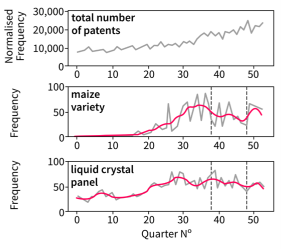
Figure 1: Time series for all three million patents, as well as samples for the main terms “maize variety” and “liquid crystal display”
Source: Office for National Statistics – Discovering emerging terminology in large text datasets using pyGrams
Notes on Figure 1:
- The grey line is the raw series.
- The magenta line is a smoothed version of the raw series using the Kalman filter.
- The main term graphs show a representative example for the levels of noise and volatility in the patent dataset.
Emergence scores
We analysed the time series data by identifying and ranking emerging terminology by assigning an emergence score. We explored two different methods for calculating the emergence score using the time series matrix: the Porter (2018) e-score and the return rate of smoothed time series with Kalman filter (net growth).
The first method is a state-of-the-art approach in technological forecasting. This method was recommended by the project stakeholder, the Intellectual Property Office (IPO). The net growth method is commonly used in economics time series analysis. The patent team developed this method as an alternative to allow flexibility on the analysis period range that was not available using Porter’s methodology.
Porter’s e-score
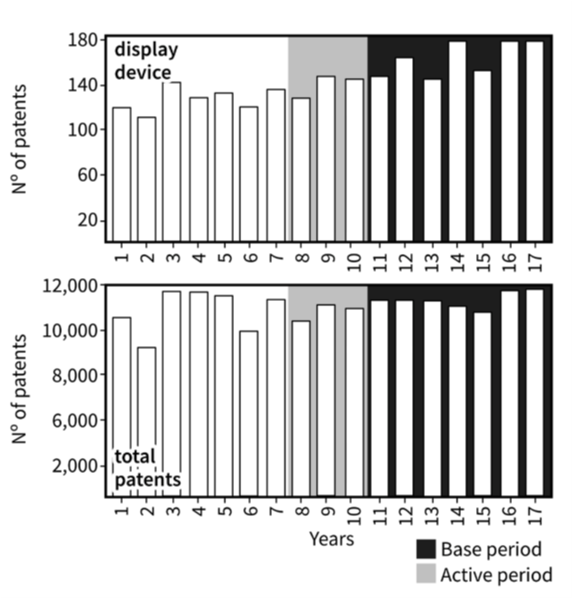
The team attempted to replicate the emergence scores reported by Porter (2018). This method derives an emergence index based on 10 periods. This is defined as 10 quarters of time series data (Figure 2). The first (oldest) three data points are defined as the base period. The following seven data points are defined as the active period. To perform emergence calculations, the total term count in the active period must be at least twice the term counts in the base period. For example, for “semiconductor device”, the term must be used at least 20 times in the active period if it was used 10 times in the base period. In addition, all calculations are normalised by the global trend (Figure 1), which is the total number of documents (patents in our case) for the corresponding period.
Figure 2: Visualisation of Porter’s periods selection
Emergence is computed between periods 11 and 17 for the term “display device”
Source: Office for National Statistics – Discovering emerging terminology in large text datasets using pyGrams
The emergence score using Porter’s method can be calculated using equations one to four;
\(\)
\( A_{trend} = \frac{\Sigma_{i=8}^{10} C_{i}}{\Sigma_{i=8}^{10} \sqrt{T_{i}}} \, – \, \frac{\Sigma_{i=4}^{6} C_{i}}{\Sigma_{i=4}^{6} \sqrt{T_{i}}} \)
\( R_{trend} = 10 * \left( \frac{\Sigma_{i=9}^{10} C_{i}}{\Sigma_{i=9}^{10} \sqrt{T_{i}}} \, – \, \frac{\Sigma_{i=7}^{8} C_{i}}{\Sigma_{i=7}^{8} \sqrt{T_{i}}} \right) \)
\( S_{mid} = 10 * \frac{\left( \frac{C_{10}}{\sqrt{T_{10}}} \, – \, \frac{C_{7}}{\sqrt{T_{7}}} \right)}{10-7} \)
\( \text{e score} = 2 * A_{trend} + R_{trend} + S_{mid} \)
where i is the period number in Porter (2018), ci is the number of documents (patents) that include the relevant term for period i, and Ti is the total number of documents for period i. Equations one to three calculate the active period trend (Atrend), the base period trend (Rtrend), and the mid-to-last-period trend, (Smid) respectively. Equation four calculates the emergence score using Porter’s method, hereafter in this report referred to as the e-score.
The inclusion of Smid indicates that e-score positively weights term usage in the last three periods more than its use in the previous periods. Porter’s method should therefore be good at identifying fast-emerging terminology at the end of the time series. In pyGrams, if the total number of time series periods is greater than 10, the e-score window location can be defined by the user. By default, it is applied at the tail end of the time series. That is, the 10 most recent periods in the time series.
One limitation of Porter’s method is this fixed 10-period window. In practice, technology emergence may occur faster, or slower, than a 10-period window. Therefore, bigger or smaller windows may help identify such technologies. In addition, owing to the lack of a normalisation mechanism, this approach may favour terms with higher count magnitudes. For example, a term whose document counts are in the range of 100 to 500 will receive a higher e-score to one whose range is between 10 and 50 if their time series curve is similar. As such, a more flexible emergence scoring approach is also considered by the team.
Net growth: a state-space model with a Kalman filter
The team here proposes a new state-of-the-art method for time series analysis. Net growth uses a state-space model with a Kalman filter in its local linear form. The state-space formulation assumes there exists an underlying smooth signal contaminated by noise. This approach is valid for patent data, where a technology may have a long-term signal but short-term fluctuations. Combining a state-space model and a Kalman smoothing filter, the underlying signal at each time interval can be extracted. In addition, the first derivative of the signal can be calculated, which can be used to analyse emergence. However, when compared to Porter’s method, the net growth method has considerably higher running times. On initial tests, this was approximately two seconds per series for a 55-period time series.
The emergence score function for net growth is an adjusted sum of the growth rate:
\( r(t) = \left\{
\begin{array}{l}
\frac{f'(t)}{f(t)} \text{ if } f(t) > 1\\
0 \text{ otherwise}
\end{array}
\right. \)
\( \text{net growth} = \Sigma_{t=t1}^{tn} r(t) \)
The variable t in equation five represents the periods in the time series. The adjustment term scaling to zero was introduced to avoid exploding the value of r(t) when f(t) is in the range (0,1] and to avoid divisions by zero. When the smoothing functions value is below one, it can be safely approximated to zero without reducing accuracy significantly.
Emergence score analysis
Once emergence scores for all terms are calculated, terms are ranked by their scores. The number of terms on the analysis outputs is selected by the user, as is the time series range. The terms are then categorised into “emerging” or “declining” according to their emergence scores. For e-score and net growth, a positive score indicates growth and a negative score indicates a decline.
The two methods are compared by scoring and ranking the emerging and declining terms. Since e-score requires a fixed 10-period window, to compare e-score to net growth, a 10-quarters period range between July 2014 and January 2017 was selected. January 2017 was selected, rather than the end of the series, October 2018, to avoid edge conditions. Outputs for e-score on non-smoothed series were generated to compare the effects of smoothing.
Time series with consistently low patent counts per quarter were also excluded. That is, only terms that had at least one-quarter with 40 counts were included. This threshold was chosen as preliminary tests showed that the Kalman filter smoothing did not perform well for time series where the count was zero in several periods. This is an issue the team plans to fix in future versions of the tool.
In Porter’s (2018) paper, e-score was calculated with annual periods, which may not suffer from much noise. However, they suggest that their approach can be used with any weekly or monthly time series data also. As a 10-year window would be too long to use to help spot emerging terminology in patent documents, especially in the technology sector where change happens rapidly, the team decided to select a period of 10 quarters.
2. Results and discussion
Emergence scores
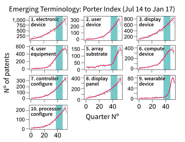
Figures 3 and 4 and Table 1 compare the 10 top-ranked emergent terms between the two methods. Only “array substrate” and “wearable device” feature in the top 10 for both methods (Table 1).
As shown in Figure 3, e-score favours terms with higher counts. Although the plot for “array substrate” has a steeper gradient than “electronic device”, “electronic device” has a larger e-score. This is caused by the difference in count magnitude between the two. “Electronic device” ranges between 700 and 1,000 counts, which is below 0.5 times growth, whereas “array substrate” ranges between 50 and 150 counts, giving it three-times growth. As shown in Figure 4, this count magnitude issue does not occur using the net growth method as the results solely reflect the uphill (or downhill) trend of each term’s slope. The absolute counts on the denominator in equation seven act as a normalisation term for net growth.
Figure 3: Top 10 emerging terms using the e-score emergence index on smoothed series
Source: Office for National Statistics – Discovering emerging terminology in large text datasets using pyGrams
Notes:
- The grey line is the raw series.
- The magenta line is a smoothed series.
- The teal box defines the date limits for assessing emergence set by the user.
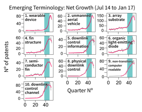
Figure 4: Top 10 emerging terms using the net growth emergence index on smoothed series
Source: Office for National Statistics – Discovering emerging terminology in large text datasets using pyGrams
Notes:
- The grey line is the raw series.
- The magenta line is a smoothed series.
- The teal box defines the date limits for assessing emergence set by the user.
Table 1 displays the top 10 ranked terms for each of the two methods. The e-score method (left) shows a tendency for more generic terms, whereas the net growth method (right) shows more specific terms to technology components. This may be because Porter’s method favours terms with higher document counts. Terms such as “electronic device” or “display device” may be a generic description of more fine-grained technologies like “unmanned aerial vehicle” or “fin structure”. Such fine-grained technologies are then highlighted using the net growth index. The ability to identify more specific, less generic, terms is important to analysts and policymakers as it can give a more refined idea of the emerging technologies.
Table 1: Emergence scores for the top 10 terms using e-score and net-growth methods
| E-score | Net growth | |||
| Rank | Term | Emergence Score | Term | Emergence Score |
| 1 | electronic device | 2.41 | wearable device | 2.655 |
| 2 | user device | 1.988 | unmanned aerial vehicle | 1.67 |
| 3 | display device | 1.832 | array substrate | 1.399 |
| 4 | user equipment | 1.430 | fin structure | 1.294 |
| 5 | array substrate | 1.352 | downlink control information | 1.0954 |
| 6 | compute device | 1.235 | organic light-emitting diode | 1.075 |
| 7 | controller configure | 1.231 | semiconductor fin | 0.959 |
| 8 | display panel | 1.104 | physical downlink control | 0.951 |
| 9 | wearable device | 1.07 | non-transitory computer readable | 0.919 |
| 10 | processor configure | 0.769 | downlink control channel | 0.840 |
Source: Office for National Statistics – Discovering emerging terminology in large text datasets using pyGrams
Notes:
- Where two terms are in common at different ranks for the two indexes, this is highlighted in blue.
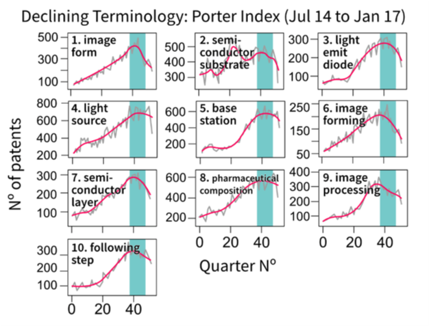
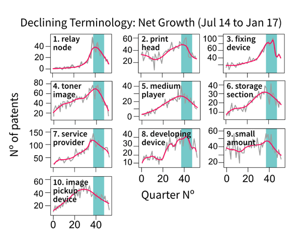
The declining e-score graphs in Figure 5 show a few terms whose smoothed curve does not have a clear declining pattern. For example, see the eighth top-ranked term, “pharmaceutical composition”. This problem was not evident in the emerging e-score graphs. In contrast, the net growth declining graphs (Figure 6) look equally as consistent as the emerging ones. Again, a difference in the patent count range for the two methods is apparent.
Figure 5: Top 10 declining terms using the e-score emergence index on smoothed series
Source: Office for National Statistics – Discovering emerging terminology in large text datasets using pyGrams
Notes:
- The grey line is the raw series.
- The magenta line is a smoothed series.
- The teal box defines the date limits for assessing emergence set by the user.
Figure 6: Top 10 declining terms using the net growth emergence index on smoothed series
Source: Office for National Statistics – Discovering emerging terminology in large text datasets using pyGrams
Notes:
- The grey line is the raw series.
- The magenta line is a smoothed series.
- The teal box defines the date limits for assessing emergence set by the user.
The difference in total counts range between the two methods is more clearly shown in Figure 7. In this figure, the patent counts for each term in the emerging top 100 ranked terms were accumulated and plotted to show the range and variance on total patent counts for the two methods.
Figure 7: Boxplot for the total counts of the time series for the same 10-period window for the top 100 emerging terms on both methods; it is evident that net growth has a lower counts range compared to e-score
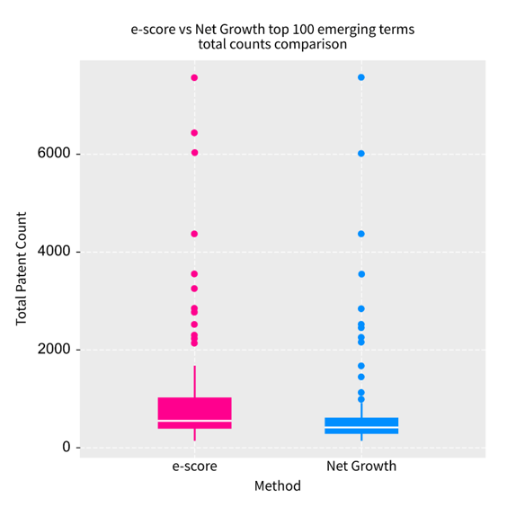
Source: Office for National Statistics – Discovering emerging terminology in large text datasets using pyGrams
Confidence: emergence score versus near future trend
This subsection focuses on how confident an analyst can be in using emergence ranking and scoring to spot emerging technologies. It discusses whether the methods described here can be used to inform decision-making for emerging technologies. To test confidence in the methods proposed here, emergence scores are compared against the trend in the following four known periods after the end date. The trend is described by the slope of the line fitted to the four future periods. To reduce any bias caused by taking a snapshot 10-period window of evaluation, we performed a 20-step sliding window across a section of our time series, also avoiding edge cases. The start period of the sliding window was June 2007. The 10-period evaluations for both emergence methods were calculated for 20 consecutive periods. That is, 10-period emergence scores plus four-period trend evaluations.
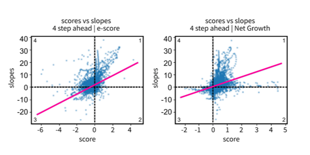
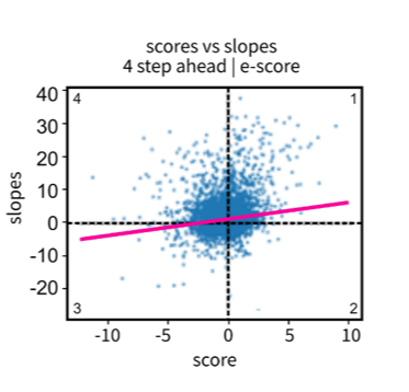
The results are plotted for emergence score versus slope with a regression line fitted (Figure 8). A good correlation would show a regression line that passes through the origin, with a positive slope. That is, one that passes through the first and third quadrants of the plots and where observations cluster the line. That would suggest the greater the score, the greater the emergence or declining slope, where the recent trend will continue in the near future.
Figure 8: Scatterplot of emergence score versus four-period ahead slope for both scoring methods: e-score (left), net growth (right)
Source: Office for National Statistics – Discovering emerging terminology in large text datasets using pyGrams
Notes:
- The e-score formula values are shifted leftwise of origin and net growth towards the right of it.
Figure 8 shows that the regression line for both methods passes through the first and third quadrants. That is, the correlation is good. In contrast, the regression line for the unsmoothed series e-scores shows a worse correlation between the scores and the future slopes (Figure 9). This supports the hypothesis that e-score works best on a smoothed time series. For e-score smoothed versus unsmoothed, more positive e-scores are calculated using an unsmoothed time series.
Data points that fall within the second and fourth quadrants show poor correlations between scores and slopes for methods. Data points in the second quadrant are time series windows with a negative score demonstrating decline, where the true future trend was uphill. Where data points fell in the fourth quadrant, the time series windows scored as emergent but the near future trend was declining.
Figure 9: Scatterplot of e-score values over a 20-step rolling window of 10-periods with unsmoothed series
Source: Office for National Statistics – Discovering emerging terminology in large text datasets using pyGrams
Table 2 gives a more quantitative overview of the results. It shows the proportion of positive scores that resulted in a positive slope and negative scores that resulted in a negative slope. The third row was a test run where some of the preliminary checks were disabled on the e-score method. Such checks include the base-to-active period ratio. As described in the Methods section, this is typically set to a value greater than two. Only a very small impact is apparent, mainly because all experiments were constrained to time series containing at least a period with 50 counts.
Table 2: Proportion of true positive hit count for both emerging and declining tasks comparison for net-growth and e-score functions
| Emerging | Declining | Total | |||||||
| All
Count |
TP
Count |
Score
(%) |
All
Count |
TP
Count |
Score
(%) |
All
Count |
TP
Count |
Overall score (%) | |
| Net-growth | 14,910 | 12,218 | 81.9 | 1,541 | 1,248 | 81 | 1,6451 | 1,3466 | 81.9 |
| e-score smoothed (no prune) | 2,658 | 2,440 | 91.8 | 13,793 | 3,722 | 27 | 16,451 | 6,162 | 37.4 |
| e-score smoothed | 2,655 | 2,438 | 91.8 | 13,652 | 3,602 | 26.3 | 16,307 | 6,040 | 37 |
| e-score non-smoothed | 6,445 | 5,142 | 79.8 | 9,342 | 2,299 | 24.6 | 15,787 | 7,441 | 47 |
Source: Office for National Statistics – Discovering emerging terminology in large text datasets using pyGrams
Notes:
- TP = true positive.
From the plots in Figures 8 and 9 and the aggregates in Table 2, several observations can be made. It is apparent that the e-score method on the smoothed time series does very well at identifying emerging terms but less well on finding declining terms. Table 2 shows that the overall hit rate, which is the number of positive-scored observations divided by the number of positive slopes. The overall hit rate for e-score (smoothed) is 92% and for net growth is 82%. However, the smoothed e-score’s sample is smaller, at 2,440 compared with 12,218 for net growth. For declining terms, net growth scored a hit rate of 82%, whereas e-score achieved only 27%. Again, the difference in sample size should be considered. These results suggest that the team’s versatile scoring function, net growth, performs equally well on both emerging and declining tasks.
The unsmoothed e-score method had more positive scores compared to its smoothed version, but the hit rate dropped to 80%, with the overall rate slightly higher at 47%. Both the smoothed and unsmoothed results show that e-score is not good at identifying declining terms. Despite its poor performance for identifying declining terms, when identifying emerging terms, the e-score method on smoothed time series performed better than net growth.
The e-score approach is normalised with the global trend (equation 6). The global time series trend has been slowly increasing for our dataset over the given range (Figure 10). This partially explains the shift of e-scores towards the left of the origin on Figure 8 and the shift of net growth towards the right.
Regarding the net growth method, we decided not to include a normalisation term for the global trend. The reason this was omitted was to broaden the scope of use for this tool. That is, the global trend is included as a feature in the time series and acts as a benchmark for the rest of the extracted terminology. For example, if at a given window the global trend has a positive score and another term scores higher, we can conclude that this term is emerging at a higher pace compared with the global trend. At the same time, the tool can also be used to understand if a time series is generally gaining counts by excluding the global trend from the equation.
Another observation is that where the e-score smoothed method has a high emergence score, there is a well-defined trend (Figure 10). This demonstrates that the larger the e-score, the greater the future slope. The e-score method gives an analyst confidence that a highly ranked terminology is likely to follow an uphill course in the near future.
Figure 10: Scatterplot and regression line for positive only scores on both methods: e-score (left) and net growth (right)
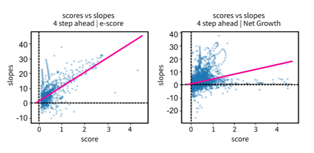
Source: Office for National Statistics – Discovering emerging terminology in large text datasets using pyGrams
3. Conclusions
This report summarises the Data Science Campus’ development of an open-source software tool to extract emerging terminology from large text datasets. The emphasis in this report was on developing a new scoring function. The team created net growth, a method based on the derivatives and smooth signal obtained from the use of a state-space model with a Kalman filter. The findings of this report suggest that this method compares very well with established methods in literature, such as e-score (Porter, 2018).
The main characteristics of e-score are the emphasis on recency and favouring terminology with greater counts. E-score performed well on identifying fast emerging terminology that is likely to continue growing in the near future but less well on declining terminology. The team’s net growth model was designed to be generalisable and was able to handle both emerging and declining terminology equally well. Our findings demonstrate net growth’s ability to judge the trend curves well. Net growth highlighted more specific terminology with lower document counts magnitude, whereas the e-score method preferred terminology with higher magnitude levels.
One of the strengths of the net growth method when compared to e-score is that it allows for more flexibility on the user-defined assessment window. In addition, it does not suffer from the constraint of 10 fixed consecutive periods to process. In the future, the team aims to make the net growth model more efficient and get feedback from stakeholders using pyGrams to identify emerging technologies in patent datasets.
Our code is freely available to use from our GitHub pyGrams repository. For more information about the tool, including examples, please visit the GitHub documents page.