pyGrams: An open source tool for discovering emerging terminology in large text datasets
Large volumes of unstructured, free-text datasets exist that can potentially hide valuable information for policymakers. One such dataset is the body of text applications for patents. A quantitative review of emerging terminology from patent applications is an important objective for the Intellectual Property Office (IPO).
For this purpose, the Data Science Campus (DSC) has developed an open source tool, pyGrams. This tool reads a text dataset as an input and produces a quantitative report of the important terms inside it. For more information visit the dedicated GitHub documents page. We have evaluated this tool with patent data. However, it will work with similar datasets such as job adverts, journal publications, coroners’ reports, survey free-text and social media free-text.
This paper describes the pipeline used to process text documents and produce time series analysis of terms, revealing emerging terminology in large datasets comprising free-text. It also presents some initial results. Alongside this publication, a more detailed report on the time series element has also been published.
We initially created pyGrams to be used by the IPO with patent data. However, it became apparent that this pipeline could be beneficial for other datasets. Such datasets include journal publications (for example, medical and statistical publications, coroners’ reports and survey free-text data). Therefore, we developed pyGrams to be able to handle any text dataset where documents and their associated date are both available.
A challenge for this project was that the candidate datasets (for example, PATSTAT, PubMed and Journals of the Royal Statistical Society) comprise millions of documents. This creates compute and memory challenges at various points in the pipeline, which is discussed in this report. The present solution consists of a text-processing step where text is embedded into a numerical document-feature sparse matrix and subsequently a feature. This feature – a time series matrix – is then persisted (cached) in disk. Then, the cached data can be queried to produce time series reports between two user-defined dates. A choice of different emergence scoring methods can also be selected.
1. Pipeline overview
Figure 1 is a flow chart of the pyGrams pipeline. This pipeline consists of several computationally intensive tasks. One such task is embedding text into a tf-idf sparse matrix for further processing. As processing large volumes of text data can take several hours, fixed parts of the process are cached after the initial run. This means the results can be reused, and it gives users the ability to run subsequent queries much faster. The green squares (white font) in Figure 1 represent processes where the end output is automatically cached. These can be read directly from permanent storage on subsequent queries. The following sections describe the pipeline and give further details for each of the steps in the diagram.
Figure 1: The pyGrams pipeline
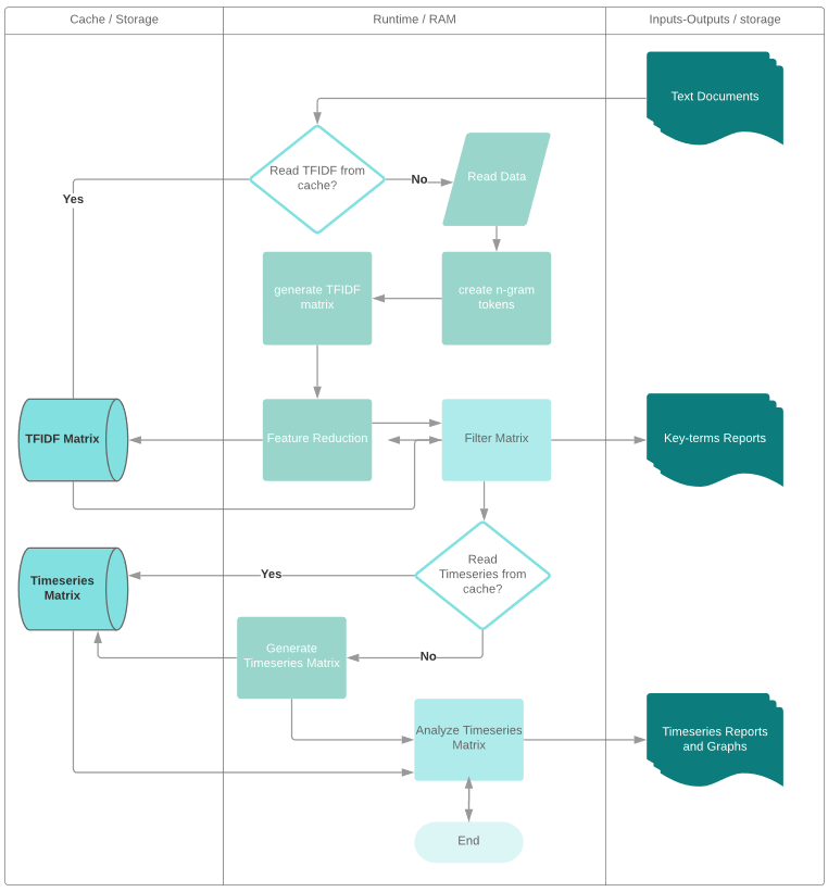
Source: Office for National Statistics – pyGrams
Notes:
- The left column shows the cached processed data, the middle column shows the processes taking place during runtime, and the right column shows inputs and outputs saved on permanent storage (for example, hard disk).
2. N-gram tokenisation
Text data are read from a free-text corpus, along with a date accompanying each document. Using standard pre-processing steps (Figure 2), each document becomes a list of n-gram tokens. N-gram tokens are defined as words or a collection of n number of words. Steps 1 to 4 are typical pre-processing tasks performed on free-text data. Step 5, lemmatisation (Plisson, Lavrač and Mladenic, 2004), is a well-known process of bringing single words into a common, human-readable base form. For example, “retrieval”, “retrieved”, “retrieves” would lemmatise to “retrieve”. An alternative to this is stemming (Porter, 1980), which is an algorithm to reduce a word to its stemmed representation. Using the same example given before, “retrieval”, “retrieved”, “retrieves” stem to “retriev”. The difference between the two, apart from readability, is that stemming is faster. This is because stemming is computed, whereas lemmatisation is slower as it is read from a dictionary. Both options are available in pyGrams for developers and may be added as user-input options in future versions.
Finally, the last part of this process is n-gram formation, which is done in two steps. First, adjacent tokens are merged to form n-grams. Then, stop words are removed to prevent undesired n-grams in the final output. Note that n-grams are not allowed to “bridge” stop words or punctuation. For example, “do this, shall” generates “do”, “do this”, “shall”. For stop words, pyGrams adopts a semi-manual approach. Inside the config directory, there are three files: stopwords_uni, stopwords_n and stopwords_glob. These files can be configured by the user. To only prevent certain uni-grams, stopwords_uni should be used. To stop certain n-grams whose order (number of terms) is greater than one (n > 1), stopwords_n is used. Finally, stopwords_glob is a stop-list that each term is stopped globally (all n-grams containing it). The file stopwords_glob is pre-populated with uni-grams from NLTK’s English stop word list.
Figure 2: Free-text pre-processing steps in pyGrams
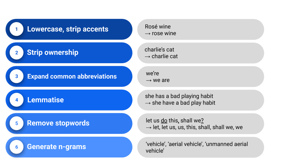
Source: Office for National Statistics – pyGrams
3. Generating a tf-idf matrix from tokenised documents
The tf-idf matrix is a well-known and established method to mine important terms from large text datasets (Spark-Jones, 1972). It does so by creating a sparse matrix of size n by m. The number of n-gram tokens (m) is given as columns and the number of documents (n) is given as row. The n-gram tokens are often referred to as a dictionary. On a large dataset, if using one- to three-word phrases (uni-, bi- and tri-grams) the count of both would be in the millions. The following equations give a brief explanation of how tf-idf is calculated for each n-gram in each document.
\( \)
\( tfidf_{i,j} = tf_{i,j} * idf_{i} \)
where, \( tfidf_{i,j} \) = tf-idf score for term \(i\) in document \(j\),
\( tf_{i,j} \) = term frequency for term \(i\) in document \(j\) and
\( idf_{i} \) = inverse document frequency (equation 2) for term \(i\), summed over all documents
\( idf_{i} = \ln \left( \frac{n+1}{df_{i}} \right) + 1 \)
where, \(n\) = number of documents, and
\( df_{i} \) = document frequency for term \(i\), summed over all documents
Sometimes, it is necessary to normalise the tf-idf output to address variable document sizes. For example, if documents comprise between 10 and 200 words, a term frequency of 5 in a 30-word document should score higher than the same term frequency on a 200-word document. For this reason, pyGrams uses the Euclidean (l2) normalisation here referred to as the l2 normalised version of tf-idf,:
\( l_{j} = \sqrt{ \strut {\Sigma_{i=0}^{m}} tf_{i,j}^{2}} \)
where the l2 normalised version of tf-idf becomes:
\( P_{i,j} = \frac{tf_{i,j}}{l_{j}} * \log \left( \frac{n}{df_{i}} \right) \)
pyGrams tf-idf calculations are based on those in scikit-learn. The user can specify the maximum (term) document frequency as a proportion of the total number of documents (argument mdf). Another important parameter in this process is the minimum document count limit, which in pyGrams is set to log(n) by default.
One of the most common problems when forming the tf-idf matrix is the relation between lower and higher n-grams of similar content in the dictionary. For example, consider the case of the tri-gram “internal combustion engine”. Its constitutional lower rank n-grams are “internal combustion”, “combustion engine”, “internal”, “combustion” and “engine”. Similar content therefore needs to be decoupled, as the scores of “combustion engine” will contribute to those of “internal combustion engine”.
One approach to this problem is to retain the score of the higher-order n-gram as a more descriptive term. That is, the counts of the higher-order n-gram are subtracted from that of the lower-order one. The rationale is that whenever a higher-order n-gram token is formed, its lower n-grams are formed as well.
This approach, however, would favour higher-order n-gram tokens. That is, if the dictionary consisted of uni-, bi- and tri-grams, only tri-grams would be kept for similar content. This would be the case if the tf-idf matrix is calculated with no lower document count limit. Conversely, the probability of three words co-located together if they are not a featured term is low. Therefore, if the minimum document count limit is too large, the resulting matrix will threshold out tri-grams, and to a lesser extent bi-grams, that are not a feature. A better approach would be for the minimum document threshold to be higher for lower-rank n-grams. This will be considered in future versions of pyGrams.
4. Feature reduction
The previous section mentions that the size of the dictionary grows exponentially when higher-order n-grams are used. Therefore, the total count of both rows and columns can be in the order of millions. To improve compute times and memory usage, feature reduction can be performed in pyGrams. Importantly, this will retain a fraction of the volume of terms while still maintaining the same tf-idf scores for the most frequently occurring terms. A basic approach is to select the top k-ranked terms by mean probability, where k is user-defined and defaults to 100,000.
\( MP(w_{j}) = \Sigma_{i=0}^{n} \frac{P_{i,j}}{n} \)
However, this approach may remove newly formed emerging terminology of lower-frequency counts. Better approaches such as variance and entropy are therefore also included in pyGrams (Alajmi, Saad and Darwish, 2012; Chekima and Alfred, 2016; and Na and Xu, 2015).
\( VP(w_{j}) = \Sigma_{i=0}^{n} \frac{(P_{i,j} \, – \, \overline{P_{j}})}{n} \)
\( H(w_{j}) = \Sigma_{i=0}^{n} \left( P_{i,j} \frac{1}{\log(P_{i,j})} \right) \)
\( \forall w_{j} \in \text{Dictionary } (j = 1 \ldots m) \)
The final feature-reduction method comprises the union of the top k-ranked terms produced by all three scoring functions detailed before (equations 5 to 7). Once the features have been reduced, the tf-idf matrix is adjusted to the new dictionary. This results in a new matrix of size n by k. The new matrix is then cached to permanent storage for later reuse by additional analyses.
5. Matrix filtering
There are two options for filtering the matrix in pyGrams: column-wise (dictionary) and row-wise (documents). The latter is carried out by choosing a date range or by filtering for classification information. For example, Cooperative Patent Classification (CPC) can be used for patents. Dictionary filtering uses word vector representations. By default, pyGrams uses the GloVe 50 model (Pennington, Socher and Manning, 2014) as the default as it meets GitHub’s storage limitations (less than 100 MB). It is possible to use other models such as fasttext 300d (Mikolov et al., 2017), word2vec 200d (Mikolov, 2013) or BERT (Devlin et al., 2019) with minimum code alteration.
Figure 3: Two-dimensional representation of word vectors
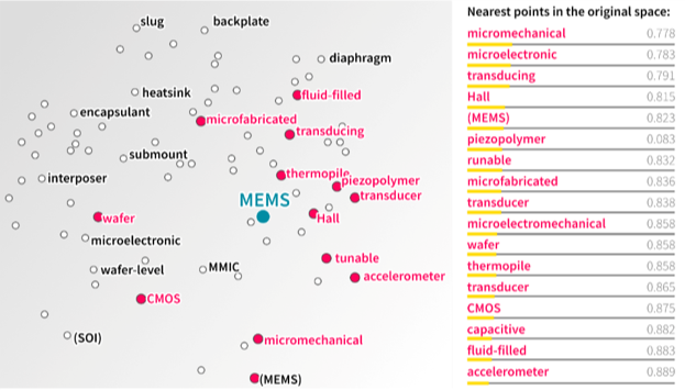
Source: Office for National Statistics – pyGrams
Notes:
- Magenta circles and labels correspond to the values in the table on the right-hand side.
The reduced dictionary and user-input terms are converted to an average word vector representation. The user also sets a threshold ratio of terms in the dictionary to keep, which defaults to 0.75. The dictionary terms are then sorted by the shortest cosine distance to the input terms vector representation. When this step is completed, pyGrams saves a report of the top-rated terms ranked by , which is the sum of their l2 normalised tf-idf score, (defined in equation 8). An example of ranked top terms, with and without filtering, is displayed in Table 1.
\( s_{j} = idf_{j} \Sigma_{i=0}^{n} P_{i,j} \)
Table 1: Comparison of top 20 terms by sum (l2 normalised tf-idf score) between filtered and non-filtered dictionary
| Normal output | Filter-words: pharmacy, medicine, chemist |
| 1. semiconductor device 3181.175 | 1. pharmaceutical composition 2446.811 |
| 2. electronic device 2974.360 | 2. medical device 847.00 |
| 3. light source 2861.643 | 3. implantable medical device 376.653 |
| 4. semiconductor substrate 2602.684 | 4. treat cancer 303.083 |
| 5. mobile device 2558.832 | 5. treat disease 291.440 |
| 6. pharmaceutical composition 2446.811 | 6. work piece 279.293 |
| 7. electrically connect 2246.935 | 7. heat treatment 278.582 |
| 8. base station 2008.353 | 8. food product 245.006 |
| 9. memory cell 1955.181 | 9. work surface 212.500 |
| 10. display device 1939.361 | 10. work fluid 202.991 |
| 11. image data 1807.067 | 11. patient body 196.159 |
| 12. main body 1799.963 | 12. pharmaceutical formulation 177.029 |
| 13. dielectric layer 1762.330 | 13. treatment and/or prevention 168.678 |
| 14. semiconductor layer 1749.876 | 14. cancer cell 159.921 |
| 15. control unit 1730.955 | 15. provide pharmaceutical comp 152.719 |
| 16. circuit board 1696.772 | 16. treatment fluid 132.922 |
| 17. control signal 1669.367 | 17. medical image 127.059 |
| 18. top surface 1659.069 | 18. medical instrument 123.362 |
| 19. gate electrode 1637.708 | 19. treatment and/or prophylaxis 114.959 |
| 20. input signal 1567.315 | 20. prostate cancer 108.456 |
Source: Office for National Statistics – pyGrams
Notes:
- The filter terms were “pharmacy”, “medicine” and “chemist”.
- The filtered terms have removed the majority of the terms as these were initially related to electronics. Instead, the top 20 terms are now related to medicines.
6. Time series matrix formation
Time series for terms are generated from the tf-idf matrix after feature reduction and filtering (if any). First, the tf-idf matrix is turned into a boolean (0 or 1) sparse matrix, which is the occurrence matrix. For each term (term j of document i),
\( t_{i,j} = \left\{
\begin{array}{l}
0 \text{ if } t_{i,j} = 0\\
1 \text{ otherwise}
\end{array}
\right. \)
The rows of the occurrence matrix (representing the documents) are sorted by date. The next step is to reduce the matrix into a time series, by aggregating the counts over a user-defined period. For example, if over one month, the term “fuel cell” had a non-zero tf-idf score for 17 documents, its count would be 17. This results in a matrix of size q by k, comprising k time series (one per term) for q periods (rows), where q ≤n.
\( ts_{k,j} = \Sigma_{i=a}^{b} t_{i,j} \)
The resulting time series matrix is also cached in permanent storage for faster access by future queries.
7. Time series analysis
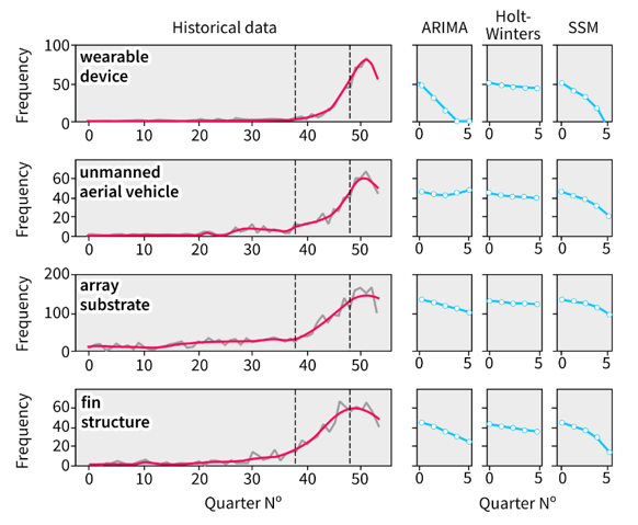
This is the final stage of the pyGrams pipeline. Here, each term’s time series vector is analysed for emergence. Then, the results are saved both visually and graphically. The analysis is carried out on a nowcasting and forecasting basis. Nowcasting is performed by first smoothing the time series using a state-space model with a Kalman filter. Then, an emergence index formula is applied to the time series between two user-defined points. The available formulas in pyGrams are the e-score index and the net-growth, developed by the pyGrams team. A separate report on state-space model suitability for this kind of time series analysis is available. Forecasting is an option in pyGrams, and the forecasting algorithms of choice are ARIMA (Perktold, Seabold and Taylor, 2019a), Holt–Winters (Perktold, Seabold and Taylor, 2019b) and state-space model (Jong, 1991). An example graphical output is displayed in Figure 4, showing the top four emerging terms. The number of terms for our outputs is user configurable and can span to hundreds.
Figure 4: Example output of the top four emergent terms scored using net-growth during the period designated by the black vertical dotted lines
Source: Office for National Statistics – pyGrams
Notes:
- Periods are quarters.
- The grey line is the raw time series.
- The magenta line is the smoothed time series using the state-space model with the Kalman filter.
- The accompanying three boxes are forecasts provided by ARIMA, Holt–Winters and state-space model for five periods (quarters) after the end of our historical series.
8. Outputs
All the outputs can be found under the “outputs” directory produced by the pipeline. These are grouped by the default file name or a user-defined one. The outputs available up to the date of publication of this document for k user-defined number of terms are:
- a ranked list of top k popular terms along with their score
- a ranked list of top k emergent terms along with their emergence score
- a ranked list of top k declining terms along with their emergence score
- time series plots of top k emergent terms in html format (Figure 4)
- time series plots of top k declining terms in html format (Figure 4)
- a graph of top k popular terms (optional)
- a graph of top k emerging terms (optional)
- a graph of top k declining terms (optional)
Graph outputs are extracted by building a graph of terms, whose initial nodes are the terms extracted by emerging or popular terminology and their top 10 co-located terms from our refined dictionary.
9. Conclusions
This report introduces a new natural language-processing tool, pyGrams, developed by the Data Science Campus (DSC). We originally developed this tool for discovering emerging terminology in patent applications for the Intellectual Property Office (IPO). However, pyGrams can be used on any structured, free-text dataset to generate trend analysis on featured terms, helping the user identify emerging terms.
The pipeline described in this report consists of three major parts: the tf-idf matrix calculation, a time series data generation from that matrix and time series analysis of this data. We have shown that by performing feature reduction and subsequent caching on the tf-idf matrix, additional analyses can be performed much quicker.
The next steps are evaluation of pyGrams by the IPO with patent data and the Office for National Statistics’s (ONS’s) Research Support and Data Access (RSDA) with Journals of the Royal Statistical Society. Following the initial evaluations, we aim to scale up pyGrams. This includes a web front end and cloud deployments. We also want to speed up tf-idf matrix calculations and Kalman filter calculations by using general purpose graphics processing units (GPGPUs). Soon, we will also publish a series of case studies where pyGrams has been a central part.
For more technical information about pyGrams, including examples and how to use the code, please visit the GitHub documents pages.
10. Acknowledgements
Patent data was obtained from the US Patent and Trademark Office (USPTO) through the Bulk Data Storage System. In particular, we used the “Patent grant full text data (no images) (JAN 1976 – present)” dataset, using data from 27 December 2004 to 1 October 2018 in XML 4.* format.