Synthetic data for public good
Government organisations, businesses, academia, members of the public and other decision-making bodies require access to a wide variety of administrative and survey data to make informed and accurate decisions. However, the collecting bodies are often unable to share rich microdata without risking breaking legal and ethical confidentiality and consent requirements.
One of the main challenges in the application of data science for public good is the lack of access to the low granularity of real-world data. This can constrain the efforts of the data science community to build robust models for organisations to make informed policy decisions and tackle major challenges such as climate change, economic deprivation and global health.
In this project, we propose a system that generates synthetic data to replace the real data for the purposes of processing and analysis. This is particularly useful in cases where the real data are sensitive (for example, identifiable personal data, medical records, defence data). Additionally, the methods developed as part of the project can be used for imputation (replacing missing data with substituted values) and augmentation of real data with synthetic data, to build robust statistical, machine-learning and deep-learning models more rapidly and cost-effectively. To generate synthetic data, our system uses machine learning, deep learning and efficient statistical representations. Regarding data sources, publicly available data (open data) are used initially. Once the developed methods have matured, they will be applied to more sensitive datasets.
The outputs of this work will result in a safer, easier and faster way to share data between government, academia and the private sector.
1. Scope
This report describes our initial analysis during the first phase of the synthetic data project. In this phase, the main objectives were:
- exploration of the research area of synthetic data generation, including literature review, identification of main algorithms, selection of methods to assess the quality of the generated synthetic data and investigation of security and privacy risks
- development of a basic system for synthetic data generation
- testing of the system for publicly available data
- identification of possible datasets owned by government organisations that could constitute potential test cases for the developed system
The sections that follow describe our efforts to meet these objectives. Specifically, they discuss:
- synthetic data background, including work previously carried out at Office for National Statistics (ONS) in data synthesis
- description of the methodology we follow for data synthesis and presentation of the components of our system
- description of the main algorithms we examined for synthetic data generation, which were the generative adversarial networks (GANs), the autoencoders and synthetic minority oversampling (SMOTE); in a complementary report (Joshi & Kaloskampis, 2019) we give a more in-depth coverage of GANs
- details of how we implemented the previously defined algorithms
- the case study selected to test our system, which is based on a real, publicly available dataset
- how we tested our system and discussion of our findings
- conclusions and next steps
2. Background
The idea of synthetic data, that is, data manufactured artificially rather than obtained by direct measurement, was introduced by Rubin back in 1993 (Rubin, 1993), who utilised multiple imputation to generate a synthetic version of the Decennial Census. Therefore, he was able to release samples without disclosing microdata. The notion of partially synthetic data was conceived by Little (Little, 1993), who came up with the idea to synthesise only the sensitive variables of the original data.
A significant milestone in the history of synthetic data was the generation of a partially synthetic dataset-based Survey of Income and Program Participation (SIPP) by the US Census Bureau in 2003 (US Census Bureau, 2018). The first version of the dataset, which was named SIPP Synthetic Beta (SSB) version 1, was not released for public use. It took three years of further development until the fourth version of the synthetic dataset finally made it to the public release in 2007. Since then, the US Census Bureau has been regularly updating SSB, mainly by adding variables that were not synthesised in earlier versions and incorporating modelling improvements. The synthetic dataset has currently reached version 7, which was released in December 2018.
As mentioned previously, Rubin’s first attempt to generate synthetic data in 1993 used multiple imputation, for which parametric modelling was employed. (Drechsler & Reiter, 2011) point out, however, that it is generally hard and tedious to produce accurate models based on standard parametric approaches. Therefore, non-parametric machine-learning approaches were used, such as classification and regression trees (Breiman, Friedman, Ohlsen, & Stone, 1984), support vector machines (Boser, Guyon, & Vapnik, 1992), bagging (Breiman, Bagging predictors, 1996) and random forests (Breiman, Random forests, 2001).
With the recent developments in deep learning, deep neural networks started becoming an attractive option for the generation of synthetic data, given their ability to use big data to build powerful models. Prominent deep-learning algorithms, which have been widely used for data synthesis, particularly in the image and video domains, are the generative adversarial networks (GANs) (Goodfellow, et al., 2014) and the autoencoders (Ballard, 1987).
There is currently an increasing interest across the public sector in the development of systems capable of producing synthetic data. In December 2018, the UK Government Statistical Service (GSS) published the findings of the National Statistician’s Quality Review (NSQR) of Privacy and Data Confidentiality Methods. This work was carried out to help the GSS use the state-of-the-art research conducted by world-leading experts from academia and industry to prepare for the future and identify opportunities to improve and innovate.
A chapter of NSQR focuses on statistical disclosure control (SDC) (Elliot & Domingo-Ferrer, 2018) and investigates synthetic data generation, as data synthesis has the same goal as traditional SDC methods, that is, to release a dataset suitable for processing and analysis while maintaining data subject confidentiality. This work gives an overview of methods for data synthesis based on traditional machine learning; however, it does not mention the latest methods using deep learning.
In January 2019, Office for National Statistics (ONS) published the findings of a pilot study that investigated the demands and requirements for synthetic data and explored various off-the-shelf synthetic data generators (Bates, Špakulová, Dove, & Mealor, 2018). The generators were applied to the microdata from the Labour Force Survey (LFS), the largest household survey in the UK. The study highlighted the advantages and disadvantages of each generator and emphasised on the challenges that the researchers phased during the synthetic data generation process, which were the choice of parameters for each generator and missing values in the original data.
In this report we present a complete system for synthetic data generation. Given the complexity of the datasets handled by ONS and the findings of the ONS methodology pilot, which highlight that often a custom solution is required rather than off-the-shelf packages, the synthetic data generator of our system provides custom solutions based on suitable models, which are learned from the original data. These models use both traditional machine-learning methods and the latest developments in deep learning.
3. Methodology
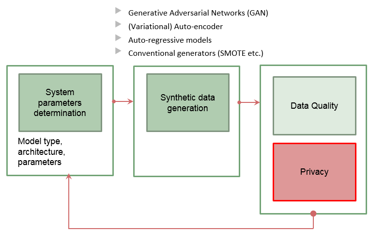
We develop a system for synthetic data generation. A schematic representation of our system is given in Figure 1. In the heart of our system there is the synthetic data generation component, for which we investigate several state-of-the-art algorithms, that is, generative adversarial networks, autoencoders, variational autoencoders and synthetic minority over-sampling. Our system operates as follows:
- first, the parameters of the synthetic data generator are given some initial values
- second, the synthetic data generator is trained on the real data using the initial parameters; the generator then produces a synthetic dataset
- third, the synthetic dataset produced by the generator is tested for:
- utility, that is, we determine whether the synthetic dataset is suitable for processing and analysis
- privacy, that is, assessment of the disclosure risks for the generated synthetic data; even though fully synthetic data provide protection from record linkage attacks, it is possible that an attacker could use the released synthetic values to infer confidential values for individuals in the original data
- finally, the initial parameters are updated based on the findings of the third step and we proceed to the second step
- the process is repeated until the criteria we have set for quality and privacy are satisfied
When assessing the output of our system, we consider two criteria, each of which correspond to a component in our system. The first criterion is the quality of the synthetic data, that is, how closely the data generated by our system resemble the real data and whether they are suitable for substituting the original data for processing and analysis. The second criterion is privacy, that is, we would like to ensure that the output synthetic datasets would not be disclosive, and would not contain identifiable data.
To assess whether the generated data meet the quality criterion we use established statistical measures. Our initial quality testing strategy is based on the method proposed in (Beaulieu-Jones, Wu, & Williams, 2017) and (Howe, Stoyanovich, Ping, Herman, & Gee, 2017), which involves comparing the pairwise Pearson correlations in the variables in the real data to the corresponding pairwise Pearson correlations in the variables in the synthetic data. Additionally, we work closely with our stakeholders who will determine whether the synthetic data are suitable to replace the original for processing and analysis.
Regarding the privacy criterion, we investigate mechanisms such as differential privacy (Dwork, 2006). The privacy component of our system is currently under development. Our initial research indicates that differential privacy is a useful tool to ensure privacy for any type of sensitive data. However, differential privacy involves introducing randomness into the data. Consequently, there is a trade-off between privacy and utility (that is, whether the generated data are good enough to replace the original data for analysis). This trade-off is different for each case study. To efficiently develop the privacy component of our system we have set up a collaboration with experts from the privacy and security team at Cardiff University, School of Computer Science. Initial results of this work are expected in the summer of 2019.
Figure 1: The proposed system for synthetic data generation
4. The techniques
Generative Adversarial Networks
Generative models are ones that can learn the underlying structure or representation of the real data used to train them. One of the main goals of generative models is that they generate new samples from the same distribution as the training set distribution. These deep-learning methods have received much interest in recent years. A host of generative models have been developed for a wide spectrum of applications, including generating realistic high-resolution images, text generation, density estimation and learning interpretable data representations.
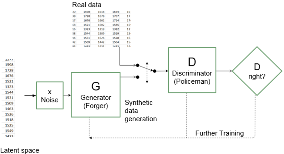
The generative adversarial network (GAN) (Goodfellow, et al., 2014) is a prominent generative model. GANs take a game-theoretic approach to synthesising new data; they learn to generate from training distribution through a two-player game. The main idea behind a GAN is to have two competing neural network models. One takes noise as input and generates samples (the generator or forger). The other model (the discriminator or policeman) receives samples from both the generator and the training data, and attempts to distinguish between the two sources. These two networks play a continuous game, where the generator is learning to produce more and more realistic samples, and the discriminator is learning to get better and better at distinguishing generated data from real data. This co-operation between the two networks is expected for the success of GAN where they both learn at the expense of one another and attain an equilibrium over time.
For a more detailed coverage of GANs, please see the complementary technical report (Joshi & Kaloskampis, 2019).
Figure 2: Overview of the generative adversarial networks
Autoencoders
The autoencoder is another popular technique for synthesising data. According to (Schmidhuber, 2015), the concept of autoencoders in the context of artificial neural networks was first presented by (Ballard, 1987). Autoencoders were originally introduced as a method for learning meaningful representations from data in an unsupervised manner.
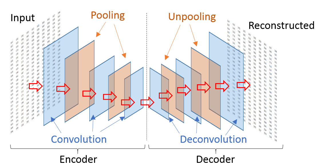
An autoencoder (Figure 3) is a feed-forward deep neural network that first compresses the input data into a more compact representation and then attempts to reconstruct the original input. The compression is achieved by imposing a bottleneck, which restricts the amount of information that travels within the network.
Due to their capacity to provide compact representations of the original data, autoencoders have been frequently used for data compression and dimensionality reduction. Compared with the widely used principal components analysis (PCA) (Pearson, 1901) method for dimensionality reduction, autoencoders are considered more powerful as they can learn nonlinear relationships, while PCA is restricted to linear relationships.
The autoencoder’s deep network consists of two individual deep neural networks. The first of these networks is called the encoder and compresses the input data into a short code. The second deep network is called the decoder; it is a mirror image of the encoder and its purpose is to decompress the short code generated by the encoder into a representation that closely resembles the original data.
Figure 3: Structure of a typical autoencoder used to generate synthetic data
We also consider a more modern version of autoencoders, called variational autoencoders (VAEs) (Kingma & Welling, 2013). VAEs use the same architecture as autoencoders but impose added constraints on the learned encoded representation.
Synthetic minority over-sampling
Synthetic Minority Over Sampling (SMOTE) synthesises new data instances between existing (real) instances and was developed to help address the problems with applying classification algorithms to unbalanced datasets. The technique was proposed in 2002 (Chawla, Bowyer, Hall, & Kegelmeyer, 2002) and is now an established method, with over 85 extensions of the basic method reported in specialised literature (Fernandez, Garcia, Herrera, & Chawla, 2018). It is available in several commercial and open source software packages. A way to visualise how the basic concept work is to imagine drawing a line between two existing instances. SMOTE then creates new synthetic instances somewhere on these lines.
Figure 4: A visual demonstration of generating new samples using SMOTE
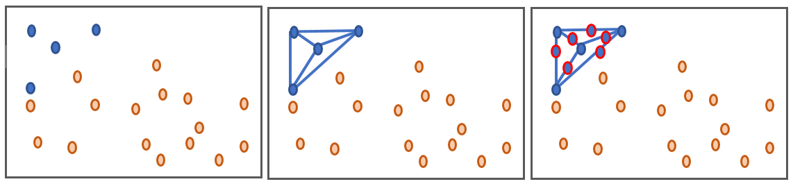
Initially there are four blue samples and 16 orange ones (far left). Lines are drawn joining the minority blue samples (centre) and new data points placed randomly on these lines (right). This has generated six new blue samples in the same data area as the original minority data.
In the example in Figure 4, we start with an imbalance of four blue compared with 16 orange instances. After synthesising it is now 10 blue compared with 16 orange instances, with the blue instances dominating within the ranges typical for the blue values. This is an important aspect of the technique – over-sampling with replacement focused data in very specific regions in the decision region for the minority class. It does not replicate data in the general region of the minority instances, but on the exact locations. As such, it can cause models to overfit to the data.
Considering a sample , a new sample will be generated considering its k nearest neighbours. The steps are:
- take the difference between the feature vector sample under consideration and its nearest neighbour
- multiple the difference by a random number γ between 0 and 1 and add this to the sample vector to generate a new sample

Variations of the technique have been developed by varying the way the samples and their neighbours are selected ahead of generating new ones. The imbalanced-learn library API offers regular SMOTE, Borderline1 and Borderline2 variants and the related Adaptive Synthetic interpolative technique (ADASYN) (Haibo, Bai, Garcia, & Li, 2008). These techniques will offer small variations in how the data are synthesised based on the distribution of the data. All were used in the study to understand which variant performs best for different datasets.
5. Implementation
The code for the synthetic data project was written in Python 3. We first applied several pre-processing steps to the dataset, including removal of incomplete data and normalisation.
Autoencoders and variational autoencoders were then applied as follows:
- the implementation of autoencoders and variational autoncoders was written in Keras and Tensorflow
- a fraction of the original data was used to train the autoencoders or variational autoencoders; training resulted in learning a representation of the original data
- the learned representation was applied to the samples of the dataset not used for training to produce synthetic data
For generative adversarial network (GANs) and WGANs, the following steps were followed:
- Keras and Tensorflow were used to build the GANs and WGANs
- the fraction of the original dataset was used to train the GANs and WGANs
- the synthetic samples were generated using the generator built at the final step of the training
The ability of synthetic minority oversampling (SMOTE) to generate numerical data was assessed using the following approach:
- take an existing dataset with n entries, make imbalanced (by replicating the dataset and assigning a target class) or generate a dataset with different features and an imbalance of 2 to 1 (this results in a generated dataset with the same number of samples at the original)
- run SMOTE (all variants) to generate new data samples (n new samples) using the imbalance_learn library
- remove new samples from new dataset
- compare against original dataset
6. Experiments and results
Dataset
To assess the ability of the different models to synthesise data we initially used publicly available datasets. Once the developed methods have matured, they will be applied to real, sensitive datasets, for example, the Labour Force Survey. However, this initial work uses open (non-sensitive) data to test the methodology openly and without privacy constraints.
The main focus of testing was the US Adult Census data available from the UCI repository (Kohavi & Becker, 1996). The dataset is initially designed for a binary classification problem, that is, to predict whether the income of an individual exceeds $50,000 per year based on census data. It has 30,162 records and consists of a mixture of numerical and categorical features including: age, working status (work-class), education, marital status, race, sex, relationship and hours worked per week. The full list of features is shown in Table 1.
The continuous variable “fnlwgt” represents final weight, which is the number of units in the target population that the responding unit represents. It is used to weight up the survey results and it is not intrinsic to the population, but an external variable that is dependent on the sample design. However, for the sake of the present analysis we do treat this variable as a “normal” feature and train our GANs on the complete dataset.
Table 1: List of the features of the US Adult Census dataset
| Variable name | Type | Description |
| age | numerical | Age |
| workclass | categorical | Type of employment |
| fnlwgt | numerical | Final weight, which is a sampling weight |
| education | categorical | Level of education |
| education.num | numerical | Numeric representation of the education attribute |
| marital.status | categorical | Marital status |
| occupation | categorical | Occupation |
| relationship | categorical | Relationship status |
| race | categorical | Ethnicity |
| sex | categorical | Gender |
| capital.gain | numerical | Income from investment sources, apart from wages or salary |
| capital.loss | numerical | Losses from investment sources, apart from wages or salary |
| hours.per.week | numerical | Worked hours per week |
| native.country | categorical | Native country |
In this report, we present results for the numerical features of the US Adult Census dataset (Figure 4). The study of categorical data will be the subject of future work. Preliminary results for synthesising categorical data using generative adversarial networks (GANs) are available (Joshi & Kaloskampis, 2019).
Figure 5: Snapshot of the numerical variables of the US Adult Census dataset
| Age | final_weight | education_num | capital_gain | capital_loss | hours_perweek | |
| 26935 | 48 | 236858 | 7 | 0 | 0 | 31 |
| 9830 | 18 | 374969 | 6 | 0 | 0 | 56 |
| 22587 | 58 | 280519 | 9 | 0 | 0 | 40 |
| 6786 | 39 | 114079 | 12 | 0 | 0 | 40 |
| 25191 | 39 | 193689 | 10 | 0 | 0 | 40 |
| 9766 | 34 | 189759 | 13 | 0 | 1977 | 45 |
| 24135 | 25 | 220220 | 7 | 0 | 0 | 45 |
| 22718 | 53 | 139671 | 10 | 0 | 0 | 40 |
| 21127 | 25 | 209286 | 10 | 0 | 0 | 40 |
| 13143 | 28 | 154863 | 13 | 0 | 0 | 35 |
Quality measures
Quantitative quality measurement
Our initial quality testing strategy is based on the method proposed for the problem of synthetic data generation in (Beaulieu-Jones, Wu, & Williams, 2017) and (Howe, Stoyanovich, Ping, Herman, & Gee, 2017). The logic behind this method is to determine whether the relations between the variables in the original data are preserved in the synthetic data. To assess the quality of the generated synthetic data we proceed as follows.
We first evaluate the pairwise Pearson correlation between the n variables observed in the real data. The results are stored in the nxn matrix PCorrreal.
Then, we evaluate the pairwise Pearson correlation between the n variables in the synthetic data and the n variables observed in the real data. The results are stored in the nxn matrix PCorrsynth.
We investigate whether the Pearson correlation structure of the real data is closely reflected by the correlation structure of the synthetic data. To achieve this, we define PCorrdiff as follows:
PCorrdiff = PCorrreal – PCorrsynth
For a synthetic dataset of good quality, PCorrdiff should be close to zero. We present PCorrdiff matrices for all synthetic data generators in the form of diagonal correlation heatmaps.
Finally, we compute the mean of the absolute values of PCorrdiff for all generators, µabs which serves as a concise quantitative measure of synthetic data quality.
The metric µabs captures the proximity between the real data and the synthetic data. Therefore, lower values of µabs represent higher accuracy. The same applies for the matrices PCorrdiff.
Qualitative quality measurement
To qualitatively assess the quality of the generated synthetic data, we observe their proximity to the real data. To achieve this, we plot the pairwise relationships of the variables in the dataset for all tested synthetic data generators and we compare them to the corresponding relationships occurring in the real data.
Hyperparameter optimisation
We optimised the hyperparameters of the algorithms we used for synthetic data generation against the aforementioned µabs metric with grid search. Note that the optimisation process for the deep-learning models is still in progress, as we are currently experimenting with different types of neural networks to further improve performance.
For autoencoders, a symmetrical model with two hidden layers (one for the encoder and one for the decoder), 15 hidden neurons, batch size of 128, 5000 epochs and 0.01 learning rate yielded the best result with respect to the evaluation metric.
The best performing variational autoencoder had two hidden layers (one for the encoder and one for the decoder), 15 hidden neurons, batch size of 128, 5000 epochs and 0.075 learning rate.
Regarding GANs, after thorough hyperparameter tuning, we found that a deep model with three fully connected hidden layers, 15 hidden neurons, batch size of 64, 5000 epochs and 0.0005 learning rate offered the best results.
The best results for WGANs were obtained with a model with three fully connected hidden layers, 15 hidden neurons, batch size of 128, 5000 epochs and 0.00005 learning rate.
Synthetic minority oversampling (SMOTE) does not require parameter optimisation.
Results
The quantitative results from our experiments on synthetic data generation with several methods are summarised in Table 1 and Figure 6. Note that, because the metrics µabs and PCorrdiff capture the proximity between the original and synthetic datasets, lower values of the metrics correspond to higher accuracies. Additionally, the results presented here are specific to the US Adult Census dataset and we are uncertain whether they generalise.
All tested methods produced high-quality synthetic samples as the Pearson correlation structure of the real data was closely reflected by the correlation structure of the synthetic data. It is evident that SMOTE and autoencoders perform best. On the other hand, the variational autoencoders produced the least accurate result, which can be improved with further optimisation. Regarding the performance of GANs and WGANs, while these models performed worse in this example than autoencoders and SMOTE, their generator is completely detached from the real data. Thus, they can be used in conjunction with mechanisms such as Differential Privacy to produce synthetic data with strong privacy guarantees.
The qualitative assessment of the quality of the generated synthetic data is based on visualising the pairwise relationships of the variables in the dataset and given in Figure 7 for the methods that performed best in the quantitative accuracy benchmark, that is, SMOTE and autoencoders. In concision, we present the pairwise relationships of a single variable (age), with the rest of the variables observed in the dataset. It is observed that all tested methods have produced synthetic data of close proximity to the real data.
It should be noted that we have worked with established statistical measures which give an indication regarding the quality of the generated synthetic data. Further quality metrics are presented in the complementary technical report. In practice, however, the stakeholders may, according to their needs, decide on utilising additional metrics, which can be specific to the properties of the original data, to determine whether the synthetic data are suitable to replace the original for processing and analysis.
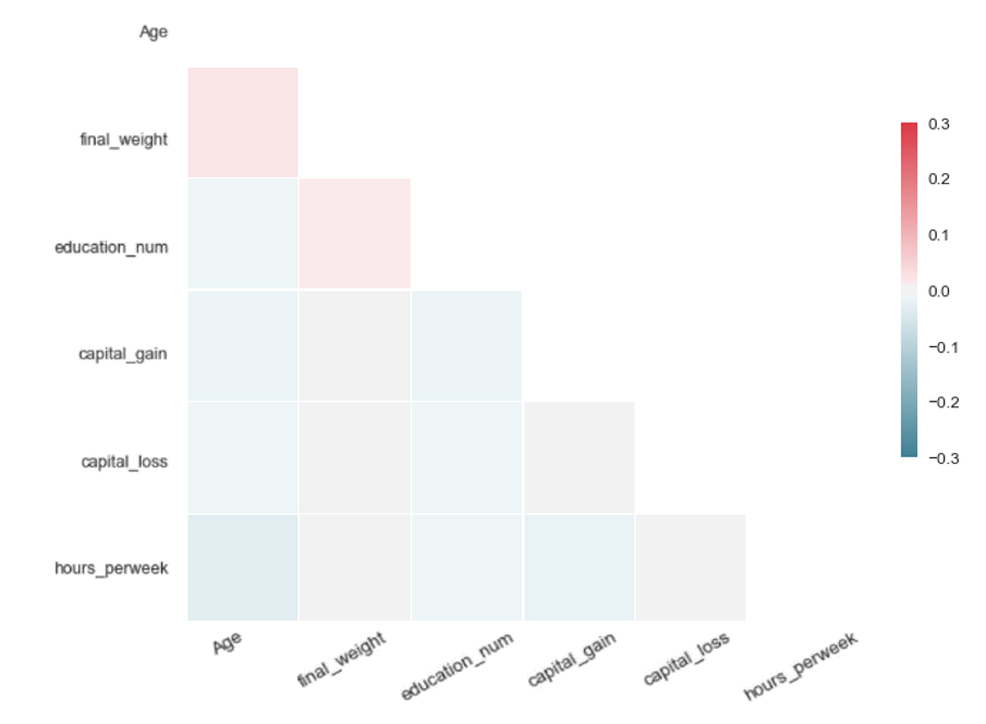
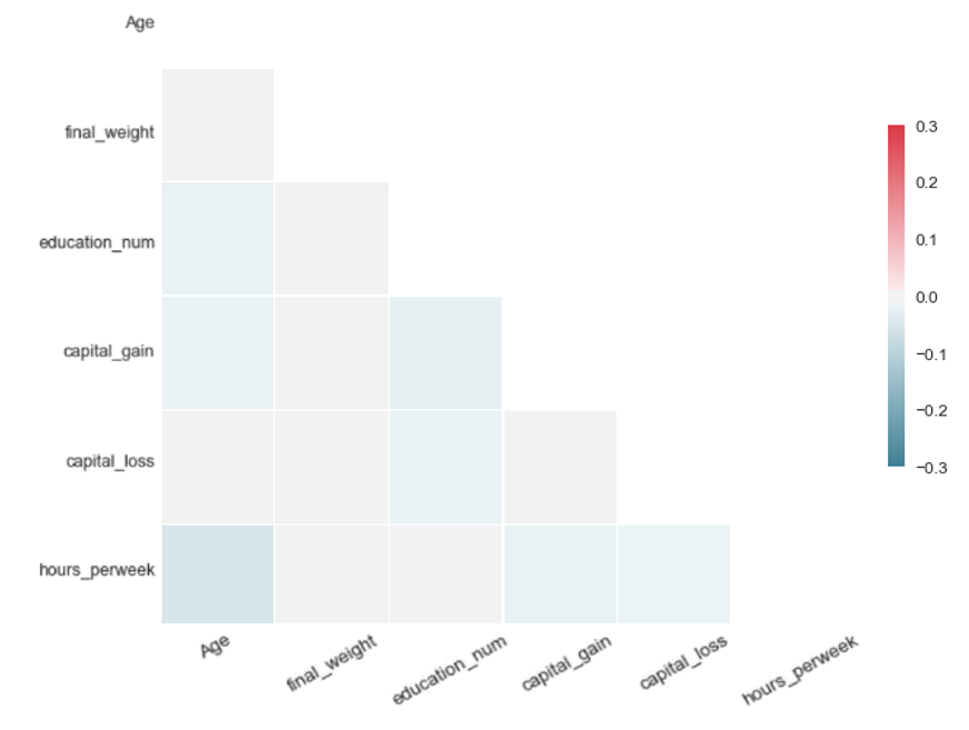
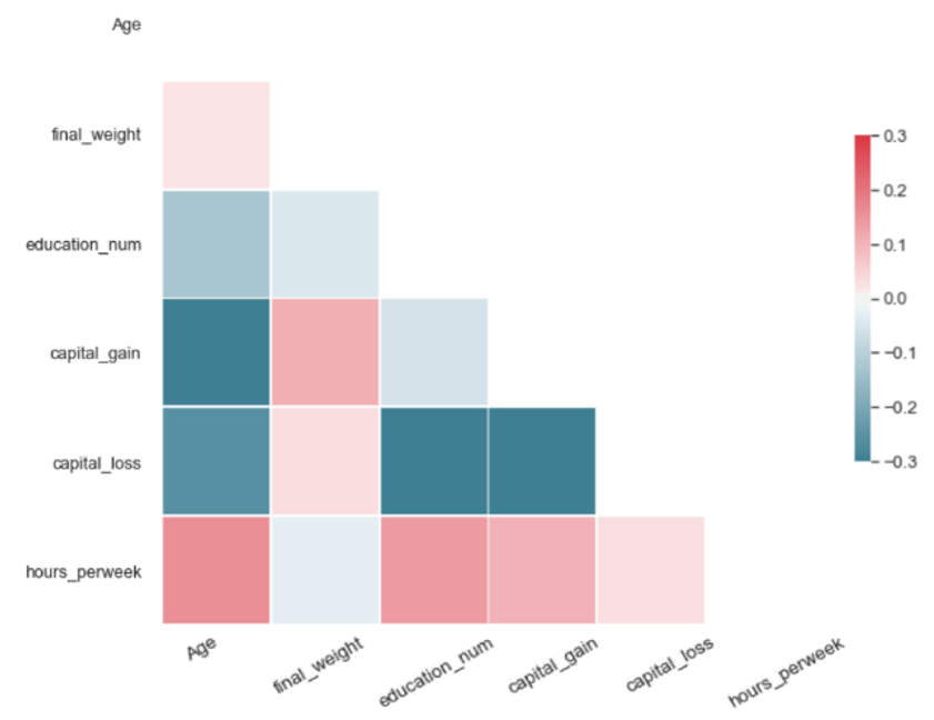
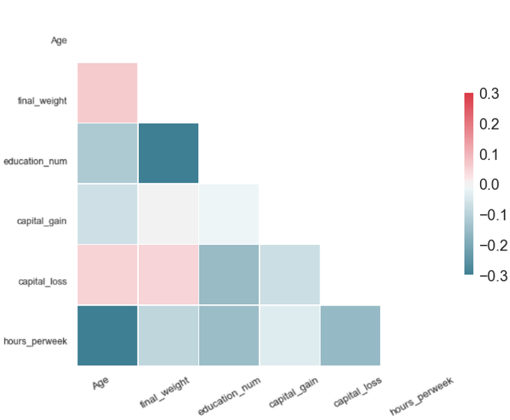
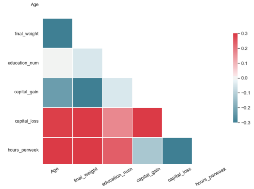
Table 2: Data quality assessment: diagonal correlation matrices in the form of heatmaps for the synthetic data generators tested by our team on the US Adult Census dataset
| SMOTE | SMOTE ADASYN |
 |
 |
| GAN | WGAN |
 |
 |
| Variational Autoencoder | Autoencoder |
 |
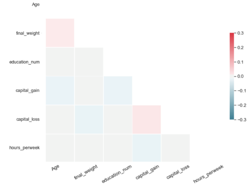 |
| Each matrix illustrates the difference of the pairwise Pearson correlations between the real and the synthetic data for the corresponding algorithm. Values close to zero indicate closer proximity to the original data. Therefore, SMOTE and autoencoders offer higher accuracy in data synthesis in our experiment. | |
Figure 6: Results for synthetic data generation for the US Adult Census dataset
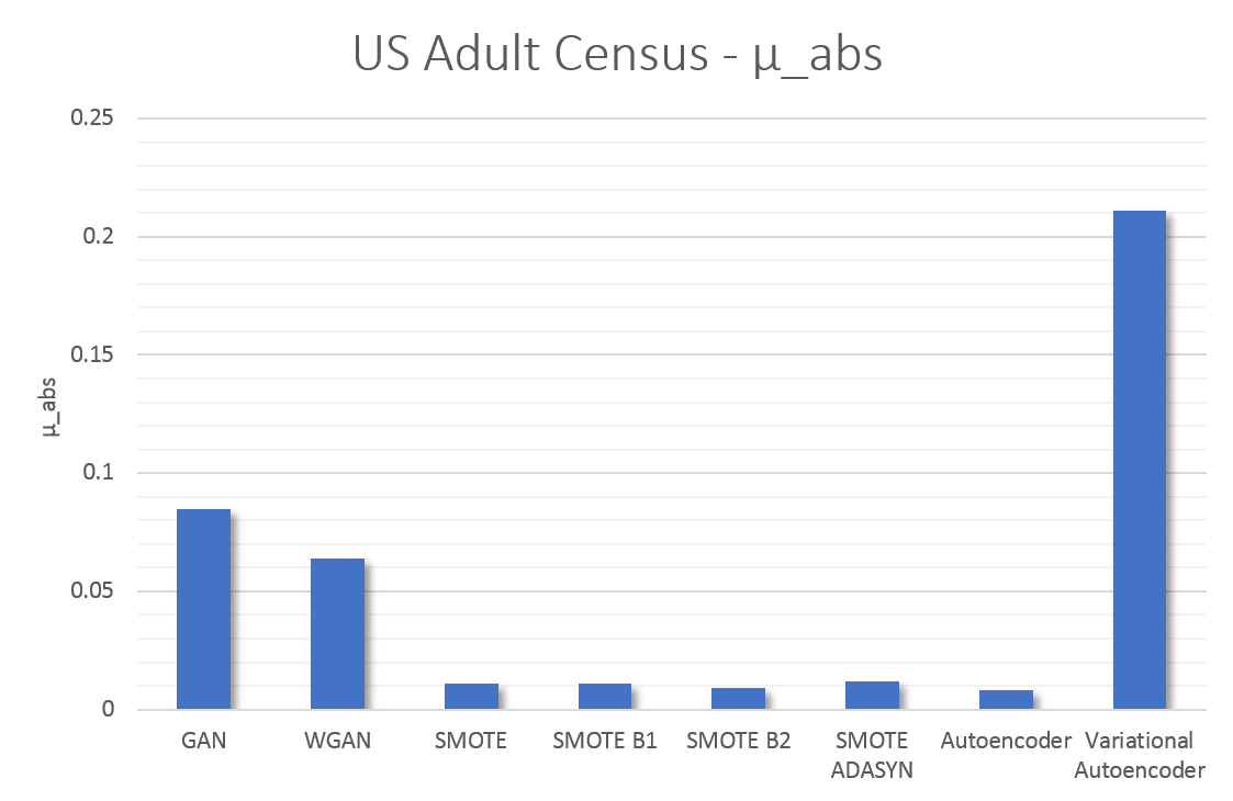
The metric µ_abs measures the proximity between the real and the synthetic data for each algorithm and, consequently, values closer to zero indicate closer proximity to the real data. According to µ_abs, in our experiment, SMOTE and autoencoders offer higher accuracy in data synthesis in this case.
Figure 7: Qualitative data quality assessment
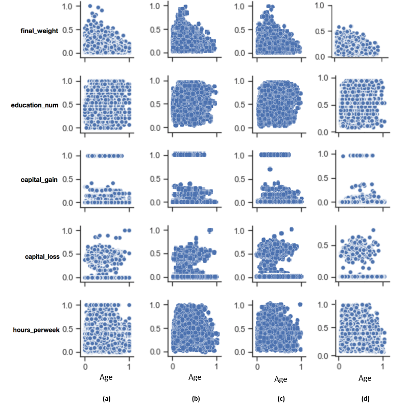
1. (a) refers to real data, (b) refers to SMOTE, (c) refers to SMOTE ADASYN, and (d) refers to autoencoders . 2. This assessment aims to visually compare the pairwise relationships between the variables observed in the real and synthetic datasets. In this diagram we plot the relationships between the variable “age” and the remaining variables of the US Adult Census dataset. It is evident that all algorithms reproduce with good accuracy the variable relationships observed in the original data.
Advantages and disadvantages
Table 3: Advantages and disadvantages of each technique for this example
| Advantages | Disadvantages | |
| GAN | Generated data are not sampled from the real data, which can give privacy properties. | Difficult to tune, can take a long time to train. |
| Autoencoder | Good results for standard hyperparameter values. | Difficult to tune, especially variational autoencoders. |
| SMOTE | Standard package, good results without the need for parameter optimisation. | Generated data are sampled from the real data. |
7. Conclusions and future work
We presented a system for synthetic data generation and experimented with several prominent techniques that are used for data synthesis. We found that the data generated by the autoencoders and synthetic minority oversampling (SMOTE) are closest to the original data as determined by our chosen data quality assessment criterion. As both of these models are relatively easy to use and tune, we recommend their use for standard synthetic data generation problems. When data privacy is a requirement, we recommend the use of generative adversarial networks (GANs) and WGANs in conjunction with privacy preserving mechanisms such as differential privacy.
Additionally, please note that this work describes the first stages of our work in data synthesis. In this report, we conducted our experiments on a dataset consisting of around 30,000 records and 15 variables, of which we focused on the numerical variables. We are aware that in many cases there is the need to synthesise datasets with millions of records and several hundreds of variables. We therefore acknowledge that further experimentation is required to draw definitive conclusions with respect to the ability of the tested algorithms to generate synthetic data.
In future work, we plan to study the generation of synthetic data for the case that the original dataset includes categorical variables. Additionally, we will incorporate privacy preserving mechanisms into our system. Finally, we intent to apply our algorithms to large-scale data.
8. References
Ballard, D. H. (1987). Modular learning in neural networks. Proceedings of the sixth National conference on Artificial intelligence (AAAI 1987), pages 279 to 284. Seattle.
Bates, A. G., Špakulová, I., Dove, I., and Mealor, A. (2018). Synthetic data pilot. In: Working paper series. Office for National Statistics.
Beaulieu-Jones, B. K., Wu, Z. S., and Williams, C. (2017). Privacy-preserving generative deep neural networks support clinical data sharing. bioRxiv 159756.
Boser, B., Guyon, I., and Vapnik, V. (1992). A training algorithm for optimal margin classifiers. Proceedings of the Fifth ACM Workshop on Computation Learning Theory (COLT), pages 144 to 152. New York: ACM Press.
Breiman, L. (1996). Bagging predictors. Machine Learning, 24, pages 123 to 140.
Breiman, L. (2001). Random forests. Machine Learning, 45, pages 123 to 140.
Breiman, L., Friedman, J., Ohlsen, R. A., and Stone, C. J. (1984). Classification and Regression Trees. Belmont, CA: Wadsworh, Inc.
Chawla, N. V., Bowyer, K. W., Hall, L. O., and Kegelmeyer, W. P. (2002). SMOTE: Synthetic Minority Over-sampling Technique. Journal of Artificial Intelligence Research 16, pages 321 to 357.
Drechsler, J., and Reiter, J. P. (2011). An empirical evaluation of easily implemented, nonparametric methods for generating synthetic datasets. Computational Statistics and Data Analysis, volume 55, issue 12, pages 3,232 to 3,243.
Dwork, C. (2006). Differential privacy. Proceedings of the 33rd international conference on Automata, Languages and Programming, pages 1 to 12. Venice, Italy.
Elliot, M., and Domingo-Ferrer, J. (2018). The future of statistical disclosure control. In: Privacy and Data Confidentiality Methods – a National Statistician’s Quality Review. Office for National Statistics.
Fernandez, A., Garcia, S., Herrera, F., and Chawla, N. V. (2018). SMOTE for Learning from Imbalanced Data: Progress andChallenges, Marking the 15-year Anniversary. Journal of Artificial Intelligence Research 61, pages 863 to 905.
Goodfellow, I., Pouget-Abadie, J., Mirza, M., Xu, B., Warde-Farley, D., Ozair, S., . . . Bengio, Y. (2014). Generative Adversarial Nets. Advances in Neural Information Processing Systems, pages 2,672 to 2,680.
Haibo, H., Bai, Y., Garcia, E. A., and Li, S. (2008). ADASYN: Adaptive synthetic sampling approach for imbalanced learning. IEEE International Joint Conference on Neural Networks (IEEE World Congress on Computational Intelligence), pages 1,322 to 1,328.
Howe, B., Stoyanovich, J., Ping, H., Herman, B., and Gee, M. (2017). Synthetic Data for Social Good. Bloomberg Data for Good Exchange Conference, pages 1 to 8. New York.
Kingma, D. P., and Welling, M. (2013). Auto-Encoding Variational Bayes. arXiv preprint arXiv:1312.6114.
Kohavi, R., and Becker, B. (1996). Adult Data Set. Retrieved from UCI Machine Learning Repository.
Little, R. J. (1993). Statistical analysis of masked data. Journal of Official Statistics, 9, pages 407 to 426.
Pearson, K. (1901). On Lines and Planes of Closest Fit to Systems of Points in Space. Philosophical Magazine, volume 2, issue 11, pages 559 to 572.
Pullinger, J. (2018, December). Privacy and Data Confidentiality Methods – a National Statistician’s Quality Review. Government Statistical Service.
Rubin, D. (1993). Discussion: Statistical disclosure limitation. Journal of Official Statistics, 9, pages 462 to 468.
Schmidhuber, J. (2015). Deep learning in neural networks: An overview. Neural Networks, pages 85 to 117.
US Census Bureau. (2018). Synthetic SIPP Data. Survey of Income and Program Participation.