Data science for the public good

1. Preliminaries

Synthetic data

A synthetic dataset contains artificially generated data as opposed to genuine, real-world data.  These artificial data are created using methods called synthetic data generators. Fitting a statistical distribution to the real data and sampling from it could be considered synthetic data generation.

Synthetic datasets are typically made to resemble a real dataset in some capacity. This resemblance is also referred to as the synthetic dataset’s fidelity. Fidelity is a sliding scale, but we can identify three broad levels:

• mock, or dummy, datasets keep the structure of the real data (for instance: column names, and data types) without retaining any of the statistical information
• low-fidelity datasets retain the structure, and each column preserves some important statistical characteristics of their real counterpart. However, they do not preserve interactions between columns
• high-fidelity datasets aim to retain both the structure, and some of the detailed statistical information present in the real data

Previous work by the ONS sets out a more detailed classification of types of synthetic data.

Mock and low-fidelity data are commonly used for testing data processing pipelines, whilst high-fidelity data can be used to test more advanced analytical pipelines. High-fidelity synthetic data can also give users a more authentic experience of working with the data. For instance, by retaining challenging features such as missing data.

Contemporary research into high-fidelity synthetic data generation (from academia and industry) often relies on deep learning solutions such as variational autoencoders and generative adversarial networks (GANs), which influenced previous work in the Data Science Campus. This sort of approach can capture nuances of the real data autonomously, but they come with significant costs: increased computational power, and a reliance on enormous amounts of training data. Most importantly for our use cases, however, they lack interpretability and often do not include any explicit privacy protections.

As an organisation, the ONS is trusted to hold sensitive data on populations and businesses to enable data-driven decision making for the public good. As a result, ensuring that synthetic data we produce is private is a priority consideration when choosing between methodologies. Previous Data Science Campus work explored privacy preserving synthetic data generation with differentially private GANs. Furthermore, the Campus team contributed to the UNECE’s guide on Synthetic Data for Official Statistics, which discussed privacy enhancing technologies and measures to assess disclosure risk.

In this report we describe how we have adapted state-of-the-art synthesis methods to generate high-fidelity synthetic data, whilst ensuring the data meets the stringent requirements of data privacy legislation, including UK GDPR and the Statistics and Registration Service Act 2007.

Differential privacy

Creating high-fidelity, realistic datasets is a challenge in and of itself, but ensuring the confidentiality of the underlying data adds another layer of complexity as these criteria are at odds. As more information about the real data is released to the generator, the closer the synthetic data can be to the original data.

However, the trade-off between fidelity and privacy means the chance of compromising someone’s privacy also increases. Our methodology, described later in this report, aims to mitigate the increased disclosure risk of high-fidelity synthesis by employing a synthetic data generator with substantive disclosure control baked in. That added protection comes from a privacy framework called differential privacy.

Differential privacy (DP) is a mathematical definition of privacy introduced in Dwork, et al. (2006) which is applied to mechanisms that act on confidential data. In the case of differentially private data synthesis, the generator must adhere to the definition of DP, not the synthetic data itself. There are many variants of DP, and the family of definitions are sometimes referred to as formally private as they provide a framework to formalise and quantify what we may mean by “private.”

We omit the finer details of DP here, but for those who are interested we recommend this very approachable video, the opening chapters of this book co-authored by Dwork, and this notice on the philosophy of DP. The following points should suffice for this report, though:

• DP describes an upper bound on the added risk to an individual’s privacy if they choose to contribute to a dataset that will be queried by a DP mechanism
• this bound represents a privacy loss budget that is primarily controlled by a parameter \(\epsilon \ge 0\). Other formal privacy definitions have additional parameters to define a budget
• smaller values of \(\epsilon\) imply stronger protection against privacy loss
• a mechanism achieves DP by adding a controlled amount of noise (set by the privacy budget) to results drawn from the data

Interpreting \(\epsilon\) can be difficult as it does not have a finite range. Privacy budgets are often advised to be \(0.01 < \epsilon < 1.1\), but much larger budgets are often used in practice. For instance, the US Census Bureau used \(\epsilon = 19.61\) to create a formally private redistricting file for the 2020 Decennial Census. DP has also gained popularity in industrial settings, including at Apple where a form of DP is used to support various iOS features. Apple uses \(\epsilon = 4\) to track users’ favourite emojis per day, or around 120 per month.

Despite being introduced almost 20 years ago, DP is still in its infancy as a statistical disclosure control (SDC) method. Other, existing methods have proven effective for decades now, and there is little incentive to change tack when the alternative requires niche expertise as well as new tooling. The ONS has previously investigated DP as a tool for publishing geographically consistent marginal tables, determining the loss in accuracy too great against the benefits of the formal privacy framework.

This project presented a good opportunity to explore the use of DP in another domain, but we needed to address the issue of interpretability. Any output would have to be approved by the risk owners of the underlying data. So, we wanted to find a solution where the formal privacy framework agreed with concepts that are already familiar to stakeholders.

As well as providing interpretability, we wanted to be transparent with our stakeholders about the limitations of DP. Often, DP is lauded as a panacea that guarantees privacy in all cases. While DP offers strong claims of protection against a litany of attacks, it does not provide an absolute guarantee of privacy. As stated above, the level of protection provided by a DP mechanism is broadly determined by the privacy-loss budget.

We have spent considerable time communicating and discussing the aptness of DP for the ONS, including its use in the face of non-DP releases and its comparisons with traditional SDC. We believe that DP provides a niche for our research while minimising risk.

2. Methodology

In 2018, the National Institute for Standards and Technology (NIST) held a competition on differentially private synthetic data generation. The winning method, now dubbed NIST Maximum Spanning Tree (NIST-MST), has since been generalised to work on any categorical dataset. This generalised method, known as MST (Maximum Spanning Tree), is what we used to synthesise the census-mortality dataset.

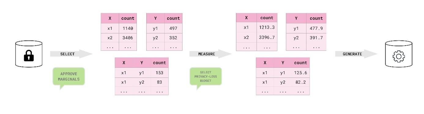
The MST method creates high-fidelity synthetic data by identifying and preserving important low-order interactions in the confidential data via a graphical model. MST consists of three major stages: selection, measurement, and generation. We omit the finer details of these stages, providing a summary of each here and paying particular attention to the selection process. Figure 1 shows a diagram of the process of creating synthetic dataset with MST, including where stakeholders could provide input into the otherwise automatic procedure.

Figure 1. Process diagram of how we applied MST with stakeholder input to synthesise the census-mortality dataset.

Being able to involve our stakeholders in the synthesis process was crucial in finding a suitable generator for this project. Their domain expertise is extremely valuable, and we were acutely aware that formally private synthesis is an emerging space, particularly in the Civil Service. Thankfully, MST ticks all our boxes.

Its success in the NIST competition demonstrates that it is among the state-of-the-art in an evolving field. In addition, MST is both adaptable and explainable to non-specialists. The graphical representation that underpins the method allows us to visualise its inner workings: we can show which interactions we will preserve, and which columns inform others.

Adaptability then follows from an explanation of the model. By sharing visualisations of how the method would synthesise the original dataset with data owners, they could review the interactions we would preserve. From there, we could include or remove any number of interactions, utilising their domain expertise without sacrificing automation.

Selection

Selection refers to the process of choosing which low-order interactions to preserve from the original data. These interactions are described as marginals, also known as contingency tables. MST includes every column’s one-way marginal in the model, and it then uses a third of the privacy-loss budget to choose a set of informative two-way marginals in a private way. The measurement step uses the rest of the budget, spending one third to measure one-way marginals and the remaining third for the selected two-way marginals.

Determining the importance of marginals

Since we know that all the one-way marginals will be included, we “measure” them first by applying a controlled amount of noise to each table. Then we create a graphical model using these noisy measurements to estimate all the two-way marginals. This interim model is created as in the generation step, described later in this section.

MST determines which two-way marginals are informative by assigning a “weight” to every pair of columns. This weight is defined as the L1 difference between the observed marginal table and the estimate sampled from our interim model. A small weight (or difference) indicates that the interim model can preserve the interaction between the column-pair without seeing it, so that pair is less important.

Choosing an optimal set of marginals

Now that we know how informative (or important) our marginals are, we must choose a set from among them to preserve; this presents two problems. First, how many pairs should we choose and, second, how do we choose them privately? The more marginals we preserve, the further we must spread our privacy-loss budget when we measure them. We also cannot choose to take the pairs with the largest weights directly because we calculated their importance using the actual counts from the confidential data, and doing so would violate the definition of DP.

We can consider this problem as a weighted graph where our columns are nodes, an edge represents the marginal between two columns, and the weight of the edge describes the importance of the associated marginal. The task is now to find the smallest set of maximally weighted edges that touches all the nodes. This set of edges and nodes describes a maximum spanning tree. If we did not care about DP, we could run  Kruskal’s algorithm now to find the maximum spanning tree of our weighted graph, but we do.

MST creates a formally private maximum spanning tree using its allotted privacy-loss budget. Working iteratively, MST randomly samples a heavily weighted edge that would connect two connected components of the graph sampled so far. The sampling stops when all the nodes have been connected. The edges of this tree are the two-way marginals we will preserve.

Augmenting selection with prior knowledge

Marginal selection can be done by hand rather than using an automated procedure. Doing so allows you to reallocate all your privacy-loss budget into measuring the marginals, meaning you can get more accurate measurements. However, it would also require significant input from domain experts both on the important relationships in the data and how the data is typically used.

We augmented the selection process to incorporate both these approaches. MST provides an efficient way of choosing a minimal set of important relationships, and we were able to share them with our stakeholders. They could then impart their domain expertise and review the selection. This review was also informed by utility analysis – or how realistic the synthetic data was.

By including the data owners in this part of the process, we (the practitioners) not only demonstrate how flexible MST is, but we also undergird the key benefits of this sort of data synthesis: that it is transparent and explainable while upholding privacy.

Measurement

Measuring a set of marginals means applying a controlled amount of noise to the cell counts in each table. The amount of noise, referred to as \(\sigma > 0\), is controlled by the size of the set and the privacy-loss budget. In MST, this noise gets applied to all one-way marginals and the selected two-way marginals. For the census-mortality dataset with \(\epsilon = 1\), we have \(\sigma \approx 56\), meaning the majority of cells in each preserved marginal are perturbed on the scale of -110 to 110, with some outliers (~5%) being perturbed more significantly. The relationship between \(\epsilon\) and \(\sigma\) is shown in Figure 2 later in this section.

Accompanying each noisy marginal is some supporting data required for generating the final synthetic dataset: the attribute(s) in the marginal, their weight, and the amount of noise added to the marginal. This weight is unrelated to the selection weight, and, by default, each attribute set has equal weight. This weight can be used to inflate the importance of certain attributes in the generation step.

Generation

Following the selection and measurement of our marginals, all the differentially private parts of the synthesis are done and there is no further interaction with the confidential data. The last step is to take those noisy marginals and turn them into a synthetic dataset.

MST relies on a post-processing tool, introduced in McKenna et al. (2019), called Private-PGM to find a suitable synthetic dataset. Due to the post-processing property of DP, the resultant synthetic dataset provides the same privacy guarantees as the noisy marginals.

Private-PGM uses a graphical model to infer a data distribution from a set of noisy measurements; its aim is to solve an optimisation problem to find a data distribution that would produce measurements close to the noisy observations. Private-PGM provides acutely accurate synthetic data for the selected marginals. It can also be used to accurately estimate marginals that were not observed directly (as in the selection step with the interim model).

The graphical model produced by Private-PGM contains the tree identified during the selection process. Private-PGM aims to achieve consistency among all the noisy marginals and may include some additional edges in the graph to increase the expressive capacity of the model. Doing so creates triangles in the graph, making it tree-like.

A key part of Private-PGM is the assignment of a direction to the edges of its graph, forming one that is also acyclic. This directed acyclic graph is then traversed from spring to sink when synthesising the columns of the dataset. We can extract this graph to demonstrate how the columns inform one another, adding to the transparency of the method.

Choosing a privacy budget

Formal privacy frameworks require practitioners to set a privacy-loss budget. To reiterate the introduction of this report, this budget defines the added risk to an individual’s privacy and is represented by a set of parameters that are difficult to interpret.

The framework to which MST adheres, Rényi differential privacy, is controlled by two parameters: the upper bound \(\epsilon\) and a cryptographically small failure probability \(\delta\). This second parameter relaxes the original definition of DP, accounting for a low-probability event that violates the bound set by \(\epsilon\). The purpose of this relaxation is to afford tighter privacy analysis to certain mechanisms.

Typically, \(\delta\) is set such that \(\delta \le \frac{1}{N}\), where \(N\) is the number of rows in the dataset. We set the parameter as:

\[
\delta = 10 ^ {-\text{ceil}\left(\log_{10} N\right)}
\]

In the above, \(ceil\) is the ceiling function. Choosing the primary privacy-loss budget parameter, \(\epsilon\), remains. This parameter controls the trade-off between privacy and accuracy for the method, so the onus should lie with the risk owners of the confidential data. Our job as practitioners is to help them make an informed decision.

Often, this trade-off is used to justify a choice for \(\epsilon\). The US Census Bureau’s choice for a high budget was driven by the end-users need for high accuracy data; they set a minimum threshold for accuracy and the Bureau found the smallest budget to satisfy that.

As our use cases do not require the data to be used to generating final statistics or analysis, this approach would be hard to implement. Not only that, but it may have inflated our privacy-loss budget to an unreasonable level. Instead, we sought to understand the criteria for other statistical releases and map our method to those. As suggested to the US Census Bureau, formal privacy parameters should be reframed using familiar notions of risk.

Through our engagement with our stakeholders, small counts stood out as a crucial point when publishing marginal tables. The ONS employs multiple statistical disclosure control methods to obfuscate small counts and preserve privacy when handling census and deaths data. The minimum count before alteration can be as high as ten, depending on the context. This definition of a small count became the basis of our approach.

MST interacts with the confidential data by taking marginal tables and adding noise to them. We agreed with the data owners that any privacy-loss budget must add noise with scale, \(\sigma \ge 10\), mirroring the largest minimum count for published datasets. Figure 2 shows the relationship between \(\epsilon\) and the \(\sigma\) applied to each two-way marginal cell for the census-mortality dataset and our \(\delta = 10^{-8}\). The theoretic curve was inferred numerically as done in applications of MST.

Figure 2. Plot of the relationship between the privacy-loss budget, \(\epsilon\), and the amount of noise added to each marginal cell, \(\sigma\). The plot also shows two critical values: the required budget to meet the minimum noise addition, and the noise added with our selected privacy-loss budget.

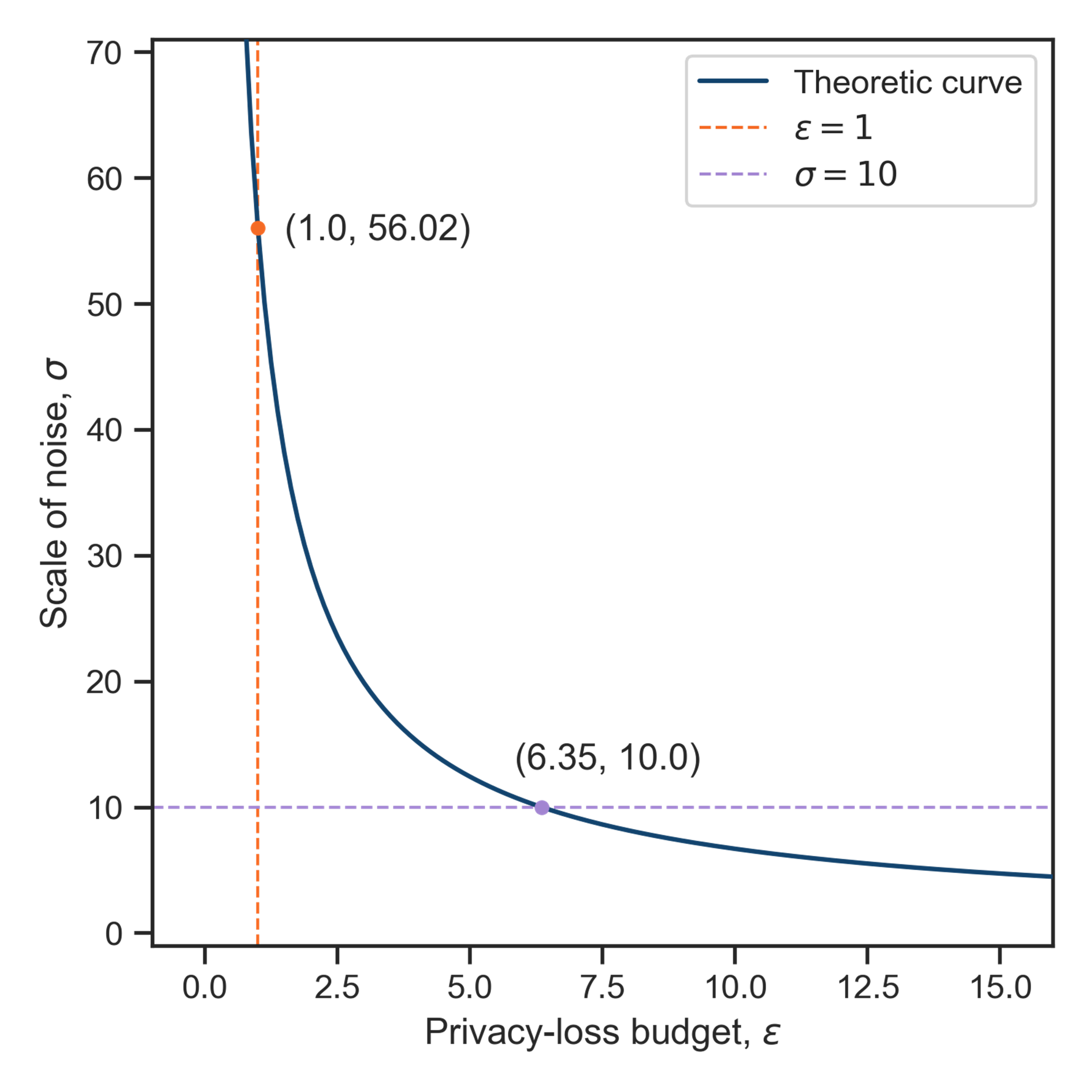
The horizontal line corresponds to our threshold of \(\sigma = 10\), which allows for a privacy-loss budget of up to \(\epsilon = 6.35\). This budget sits well beyond the academic range, but it does set an effective maximum. We synthesised datasets using a range of values for \(\epsilon\) including and beyond this maximum to assess their utility.

Despite increasing the privacy-loss budget well past our tolerance (\(\epsilon = 20\)), we saw only marginal gains in utility above \(\epsilon = 1\). For posterity, setting \(\epsilon = 1\) corresponds to \(\sigma \approx 56\), as shown by the vertical line in the figure.

Ultimately, we chose to use \(\epsilon = 1\). It surpasses our stakeholders’ minimum noise criterion generously, and it lies within the sensible range proposed by Dwork. As we were tasked with creating a general-use dataset, optimising utility was secondary.

Moreover, since the uptake of synthetic data and differential privacy are both in their infancies, we considered the level of privacy provided to be far more important. If we had a specific use case, we may have opted for a higher budget but only after exhausting any avenues to synthesise the data in a less general way.

3. Implementation

MST is a remarkably flexible method; it can accurately preserve latent relationships and requires minimal input to achieve reliable results. Plus, we have the option of fine-tuned control if we (or risk owners) want it. However, it does come with some drawbacks when attempting to scale to the size and variety of the census-mortality dataset. This section details some of those issues and how we addressed them. Broadly, these issues can be categorised into issues with scale or structures within the data.

Our implementation is available on GitHub, and it adapts parts of the original Python implementations of MST and Private-PGM developed by the authors.

An issue of scale

While the existing implementation is effective and robust, it relies on the standard open-source Python data science stack like NumPy and Pandas. These packages are limited in scale to a single machine and (natively) whatever can fit onto a single core, which was insufficient for our purposes.

The code we developed makes use of the existing implementation wherever possible, and we leverage distributed computation to handle out-of-memory tasks involving the confidential data. Reimplementing Private-PGM was considered too large a task, so we made several decisions to enable the synthesis of a large, varied dataset.

Category variety and domain size

One of the limitations in scaling MST comes from the size of the model domain. A domain records the number of unique values in each column, and its size is the product of all these counts. We handle the issue of creating a model with too large a domain in the selection process. As well as only sampling an edge that would connect two components of the tree, we exclude any edge whose inclusion would create a domain beyond what can comfortably fit in memory. We found this limit to be two billion for the census-mortality dataset.

In addition to the limit on the size of the overall domain, there are also computational limits on the size of any individual marginal. Private-PGM can only work on marginal tables that fit into memory. For our purposes, we set a limit at one million cells which filters out potential pairs in the selection process. The same limit was used by the creators in the NIST competition.

As a result, some typically important relationships are not included in the synthesis. For instance, we do not preserve the relationship between underlying cause of death ICD code and the final mention death code. These omissions will result in some confusing, unrealistic column combinations, reducing utility.

Synthesising in batches

The underlying dataset is large, containing tens of millions of rows. The existing implementation to sample tabular data from a graphical model does not scale beyond one or two million rows. Unfortunately, we were unable to reimplement a scalable version using the software available to us in the trusted research environment where we performed the synthesis. So, we had to break our synthesis into chunks.

We identified 2.5 million as the largest number of rows Private-PGM could reliably sample, and so the final dataset is comprised of many 2.5 million row chunks with any remaining rows sampled as a smaller chunk. Since each chunk is an independent sample from a single graphical model, chunking has no bearing on the privacy of the method, but it does affect its quality. For instance, the dependence structure of the rows is different from if we had taken one large sample.

In practice, we saw no discernible increase in utility between chunks of size one million and 2.5 million. Hopefully, this indicates that the improvement from whole synthesis would be negligible. However, smaller chunk sizes (in the order of tens or hundreds of thousands of rows) led to exceptionally poor univariate utility.

Inherent structures

One of the major drawbacks of MST is that it does not have a mechanism to handle structures in the data. It is a method for synthesising tabular data made up of categoric columns. The census-mortality dataset can be treated as categoric; ages and dates are continuous columns, but we still achieve good utility after casting them as categoric data types. However, the census-mortality dataset is complex and contains several inherent structures, including nested columns, group hierarchies, and structural missing values.

Avoiding internal inconsistencies

An internal inconsistency describes a logical impossibility in a dataset, like a parent being younger than their child. Avoiding inconsistencies improves the fidelity of the data by making them more plausible to a user.

Logically nested columns are common in complex datasets, and not accounting for them will lead to internal inconsistencies in the synthetic data. A set of logically nested columns would include things like truncated and detailed occupation codes or geographic areas. For instance, we synthesise Middle Layer Super Output Area (MSOA) as the lowest level of geography. We do this in part because anything lower creates a too-large marginal, but we also do not synthesise higher levels of geography.

Instead, we attach these levels (local authorities and regions) in post-processing via a lookup table because each MSOA belongs to exactly one of each higher geography. Allowing MST to synthesise any combination of these columns results in a dataset where much of the geographic data are invalid.

Another example of an internal inconsistency is breaking a structural zero. Sometimes, a zero in a marginal table means that combination is impossible; we could reframe logically nested columns as many structural zeroes. Private-PGM includes functionality to define and enforce structural zeroes but invoking this remains opaque in the implementation. As a result, we are unable to preserve structural zeroes in the synthetic dataset.

Omitting household hierarchies

MST synthesises each column as categoric, and so household identifiers would have to be treated as such. There are millions of households in the original data, so their individual marginal would be too large for MST to handle, let alone any interactions. As such, MST is not fit to handle the hierarchy between individuals and their household. We still synthesise household-level columns, however.

There do exist post-processing methods, such as SPENSER, for forming realistic households from individual-level data. Also, recent work by Cai et al. (2023) explores relational table synthesis under differential privacy. Alas, incorporating this structure is currently beyond the scope of this project.

Omitting comorbidity

The original data contains a series of final mention codes among the mortality columns. These codes describe the concurrent conditions of the individual at their time of death. This set of columns is closely entangled, and synthesising realistic combinations would be difficult.

Moreover, each code is an ICD-10 code, of which there are over ten thousand. As such, modelling their interactions would prove untenable for MST, again not even thinking about logical inconsistencies. So, we synthesise only the leading final mention code.

Health data is important for analysts, and we hope this solution offers enough value to be useful. The potential to synthesise this set of columns in a formally private way remains a matter for future work, dependent on how health data may be synthesised in the future.

Separating synthesis

The census-mortality dataset links the 2011 Census to the deaths register, and since there are far fewer deaths per year than citizens, their join is unbalanced. In fact, around 90% of all the original records belong to individuals at the Census who have not passed away. Hence, they contain no mortality data whatsoever.

This imbalance creates missing values in the data that carry meaning. Allowing MST to attempt replicating this structure dominated the synthesis. The mortality columns were synthesised first, and the structure of the graphical model did not match expectations. Moreover, the dataset performed abysmally during our generic utility analysis.

To avoid these issues, we decided to synthesise census-only and mixed records separately. We separated the dataset during pre-processing, then applied MST to each part, concatenating the resultant datasets during post-processing. The impact of this change was enormous in terms of the quality of the synthetic data, which is detailed in the next section. We still used the chunking method to synthesise each part as a series of chunks.

The obvious downside to separating the synthesis into two parts is that there are now two models to review. Thankfully, owing to the transparent nature of MST, this did not really pose a problem when communicating with stakeholders.

Figures 3 and 4 show the synthesis graph produced by Private-PGM for each part of the data: census-only records and mixed records, respectively. Each graph shows the columns as nodes and an edge indicates its inclusion in the model. A solid black edge means that two-way marginal was selected by MST, while dashed orange edges indicate a marginal included by Private-PGM to increase the accuracy of the distribution fit to the set of noisy measurements.

Figure 3. Diagram of the graphical model fit to the census-only records in the dataset.

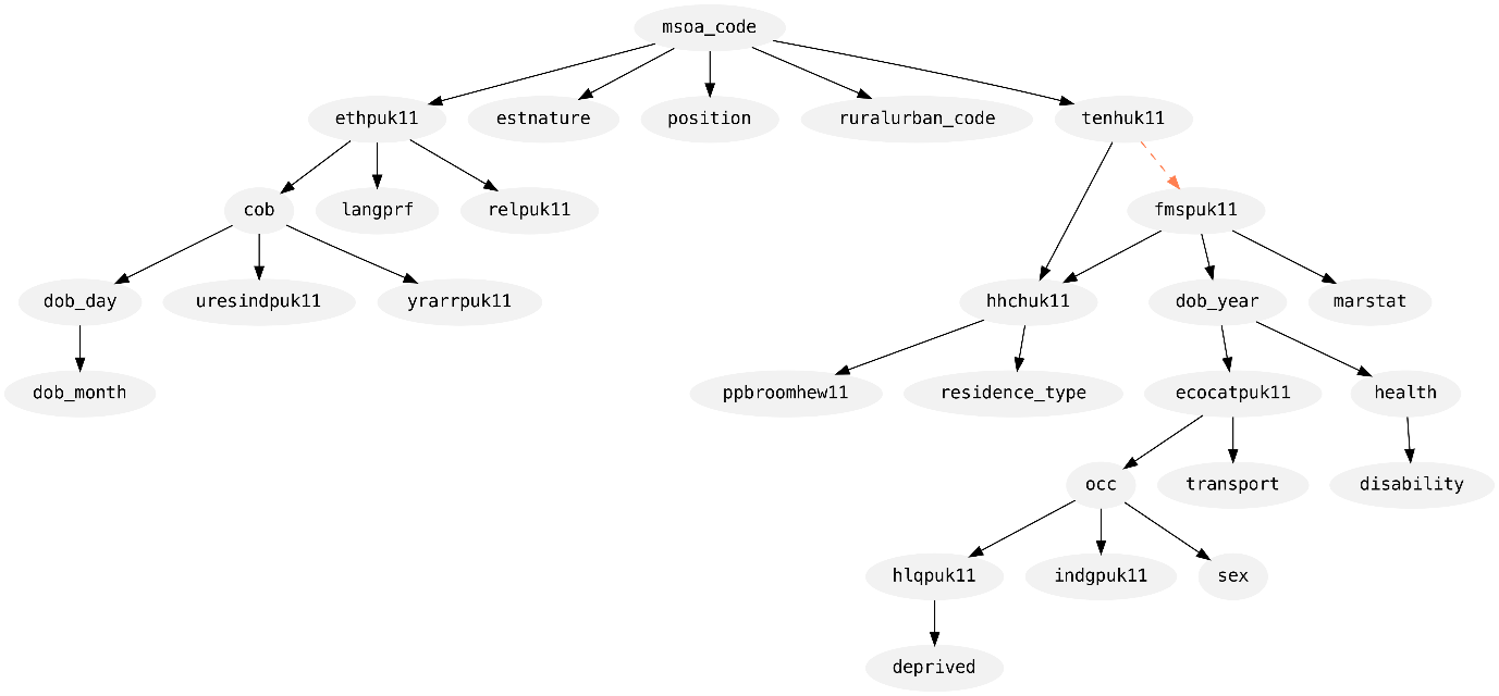
Figure 4. Diagram of the graphical model fit to the mixed records in the dataset.

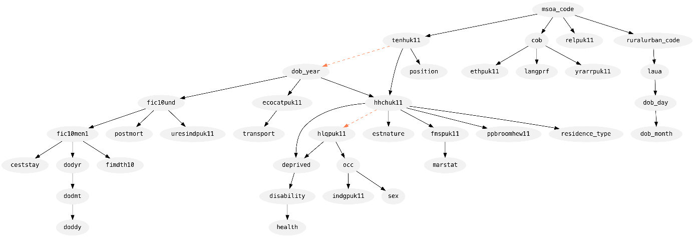
The direction of each edge is also informative here: an edge \((a, b)\) means that column \(a\) was used to synthesise column \(b\). In this way, we can see that both parts began their synthesis in the same way by synthesising MSOA at time of census (msoa_code). From there, you can follow the edges to see how each column informs the synthesis of the others.

4. Utility analysis

The utility of a synthetic dataset describes how well it represents the original data and how useful it is. Determining what it means “to represent a dataset” or “be useful” is the topic of much debate, and there are many approaches practitioners could take.

Broadly speaking, utility measures fall into one of two types: generic and specific. Generic utility measures capture how well the synthetic dataset preserves general, usually low-order, statistical properties of the real data. Meanwhile, specific utility measures describe how well the synthetic data performs at a given task compared with the real data.

For instance, you might repeat a piece of analysis with the synthetic data and compare the results with those from the original data, treating the original as a ground truth. The final task in the NIST competition was a measure of specific utility: contestants had to create a dataset that modelled the gender wage gap across various cities in the US.

When creating the synthetic census-mortality data we made use of a suite of generic utility measures and one specific utility measure.

Generic utility

There is a plethora of metrics for measuring statistical similarities between two datasets, and choosing an approach to measuring generic utility can seem like a large undertaking. We decided to separate our approach to cover three important aspects of generic utility: univariate fidelity, bivariate fidelity, and distinguishability.

Dankar et al. (2022) proposes a generalised version of this approach, swapping distinguishability for “population fidelity.” The metrics we use for univariate and bivariate fidelity mirror those used in the popular synthesis evaluation library, SDMetrics.

Univariate fidelity

Univariate, or attribute, fidelity encompasses metrics that measure the statistical authenticity of individual columns in a synthetic dataset. That is, how well formed the synthetic columns are when compared with the original. Typically, univariate fidelity measures compare fundamental aggregates (means, extrema, unique values, etcetera) or empirical distributions.

For our suite, we measure two types of univariate fidelity: coverage and similarity. Despite synthesising everything as categoric, we treat numerically encoded columns differently, using a fidelity metric that is applicable to the data type.

Coverage describes how much of the original domain is present in the synthetic column. For categoric columns, we find the category coverage: the proportion of unique categories the synthetic data produces. For numeric columns, we find the range coverage.

That is, what proportion of the original range is produced in the synthetic data. Measuring coverage is important because it demonstrates how well the generator captured the extent of the domain, and it can provide a measure of confidence in the sampling process.

Similarity is what people usually mean by univariate fidelity. We compare the empirical distributions of our real and synthetic columns depending on their data type. Numeric columns are compared via the two-sample Kolmogorov-Smirnov distance, while categoric columns use total variation distance.

The Kolmogorov-Smirnov distance (KS) compares two numeric samples, \(R\) and \(S\), by finding the maximum difference between their empirical cumulative distribution functions, denoted \(F\) and \(G\) respectively:

\[
KS(R, S) = \sup_{x \in R \cup S} \left|F(x) – G(x)\right|
\]

Total variation distance (TV) compares two categoric samples, \(R\) and \(S\), defined over the same index \(I\) by comparing their contingency tables:

\[
TV(R, S) = \frac{1}{2} \sum_{i \in I} \left|R_i – S_i\right|
\]

Both measures satisfy the definition of a distance metric and take values between zero and one. Choosing metric and scaled similarity measures is a sensible idea; they become comparable and easy to interpret. We use the complement of each of these measures so that zero indicates no similarity, while a value of one means absolute harmony.

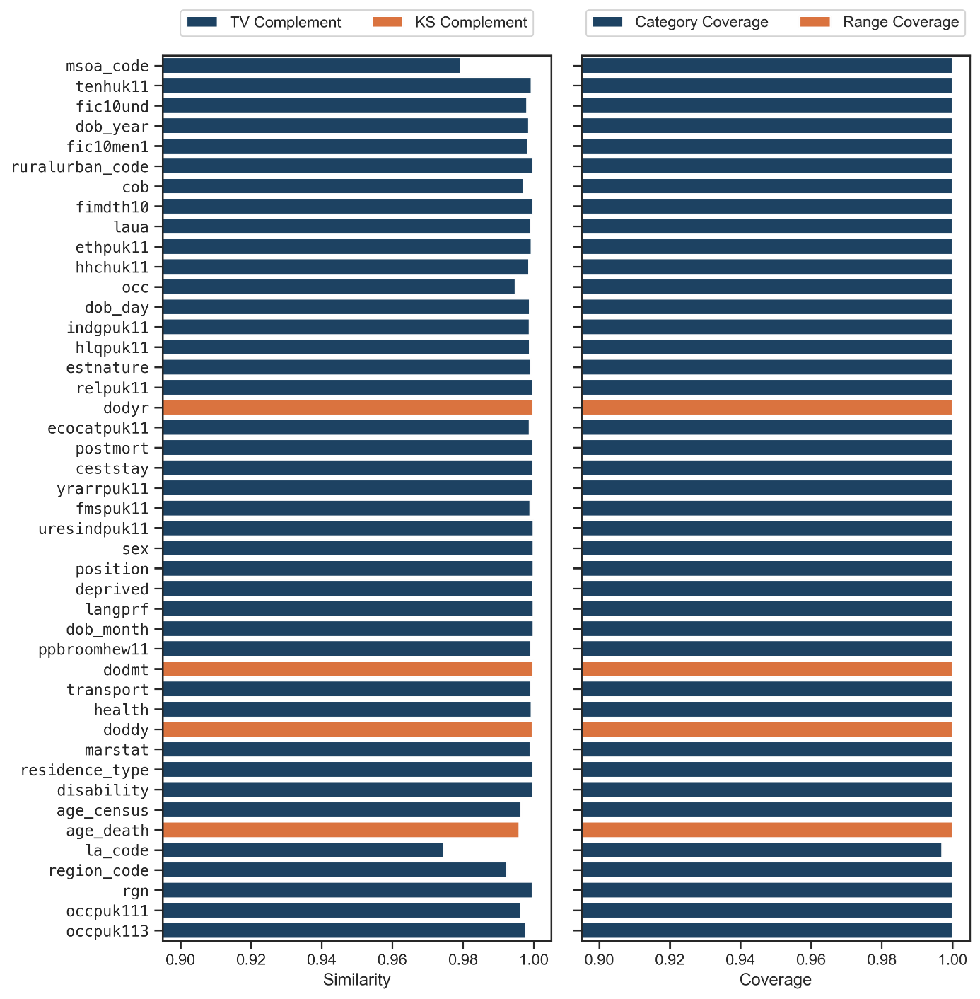
The univariate fidelity results are shown in Figure 4. Most immediate is that our synthesis preserved each column with near-perfect similarity. The same is true for the coverage for all columns except local authority at time of death (la_code). In this case, there were issues taking a fully descriptive geographic lookup table as a missing value could have multiple meanings. In all, the effect is negligible, and the similarity of the column is exceptionally high still.

Figure 5. Bar plots of univariate fidelity for each column. The left plot shows univariate similarity, while the right shows the coverage statistics.

Bivariate fidelity

Bivariate fidelity covers metrics that compare pairwise trends between the confidential and synthetic datasets. Most commonly, pairwise correlation coefficients are used. We use Spearman correlation for numeric column pairs, and total variation distance for all other pairs, discretising numeric columns first.

With a matrix of pairwise trend coefficients for each dataset, \(R\) and \(S\), we consolidate them into one bivariate fidelity matrix, \(B\):

\[
B = 1 – \frac{\left|R – S\right|}{2}
\]

The elements of this matrix take values between zero and one, where a score of zero indicates that the pairwise trend was not preserved well at all, while one indicates that it was preserved precisely. While this scoring compares the trend coefficients, it does not actually compare the pairwise relationships themselves. For instance, two numeric columns could have a strong negative correlation in both datasets, indicating high bivariate fidelity, but the shapes of the curves would not necessarily be similar.

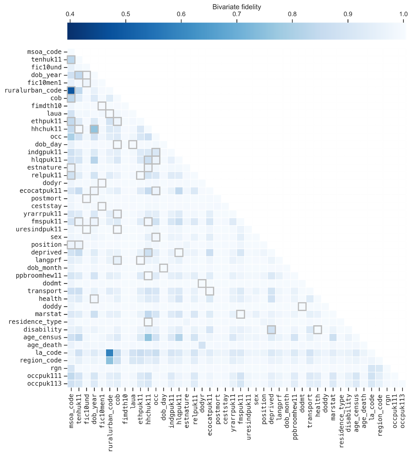
Figure 5 shows the pairwise trend comparison matrix \(B\) for the real and synthetic census-mortality datasets as a heatmap. Lighter cells indicate better preservation of that pairwise relationship.

In general, pairwise trends a very well-preserved. As we have already mentioned, one of the strengths of MST is that it can preserve low-order interactions even if they are not explicitly included in the selection or generation processes. The figure also highlights all the included marginals with a light grey border; there are many pairs that show high quality despite only being synthesised indirectly.

Figure 6. Heatmap showing the bivariate fidelity matrix for our synthetic dataset. Darker cells indicate worse fidelity. Highlighted cells show the two-way marginals chosen during the selection process.

Distinguishability

The final arm to our generic utility analysis measures the distinguishability of the synthetic data. Distinguishability indicates how well the synthetic data preserves the entire joint distribution of the original data. As such, these measures offer a good approximation of how high up the scale of fidelity your synthetic data sit.

Most often, distinguishability is measured by training a classification algorithm to tell real and synthetic records apart. The prediction probabilities from the classifier then serve as propensity scores to be summarised. Snoke et al. (2018) provides a comprehensive introduction to propensity-based utility analysis.

One issue with typical propensity score metrics is that they lack interpretability, either by being unbounded or relying on strong assumptions. For our analysis, we make use of the SPECKS method to measure distinguishability from propensity scores. The process is as follows.

1. Concatenate the real and synthetic data, appending an indicator column where zero means the record is real and one means the record is synthetic.
2. Fit a classification algorithm to the concatenated data. We used a random forest. Note that train-test splitting can be used here.
3. Extract the predicted synthetic probability from your fitted classifier. These are your propensity scores.
4. Measure distinguishability as the two-sample Kolmogorov-Smirnov distance between the real and synthetic propensity scores.

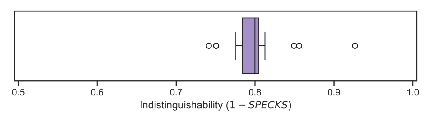
To get a more robust estimate for distinguishability, we repeated steps two through four across 20 random seeds. As with our other generic utility measures, we use the complement of these scores so that zero means the synthetic data are entirely distinguishable from the real data. The indistinguishability results can be seen in Figure 6 as a box plot. There is a tight grouping with most results sitting around 0.8, indicating that the synthetic data are difficult to tell apart from the real thing.

Figure 7. Box plot of the results to measure distinguishability. Outliers are shown as open dots.

Estimating life expectancy

We make use of one specific utility measure for our synthetic data, where we recreate an existing piece of analysis. Previously, the ONS published a report on ethnic differences in life expectancy using the 2011 Census. In the report, the authors created a table of life expectancies by sex and ethnic group, including the marginal “gaps” between those estimates. These gaps are the range of the associated column or row.

The report includes a methodology to perform probabilistic linkage since the census-mortality dataset was not readily available to analysts at the time of publishing. The fact they used a different linked dataset is immaterial as we only replicate their analysis.

That is, we calculated life expectancy by sex and ethnicity using our confidential and synthetic datasets. With these estimates, we can measure the specific utility of our synthetic data by looking at the relative difference between each estimate and gap. Figure 7 shows the results of our replicated analysis.

Figure 8. Heatmap of relative difference in life expectancy estimates by sex and ethnic group. The heatmap uses a perceptually uniform diverging colour map, where darker colours indicate more extreme values.

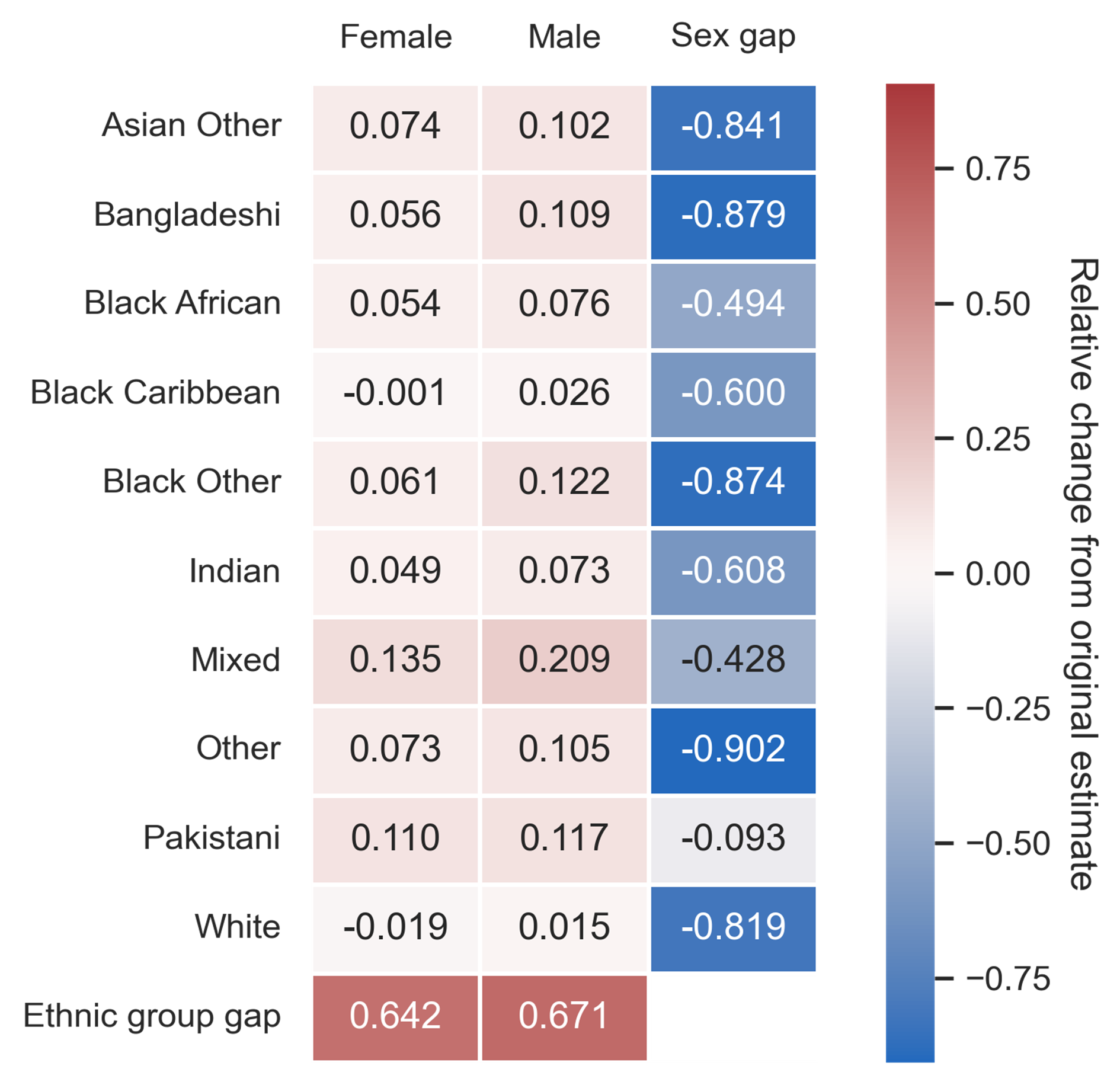
It looks like MST did a fair job at preserving individual life expectancy estimates. There appears to be a slight overestimation across groups in the synthetic data, which could be related to synthesising extreme values – an intrinsic weak spot for DP – in age. However, the gap estimates clearly did not survive the synthesis and are unreliable.

While this may appear to be a flaw in the synthetic data, why should we expect anything else? MST is a generic synthesis method, relying on a selection of low-level interactions. To explicitly preserve life expectancy by sex and ethnicity, you would need to define a six-way marginal, a task too large for MST to handle. And yet, our methodology preserves the individual estimates.

If we knew the dataset would be used to replicate life expectancy gap estimates, we could attempt to alter our selection process. There could be hope in explicitly including any two-way marginals from the six-way relationship in the synthesis models, but we leave that experiment for further work.

5. Conclusion

Our exploration into explainable, formally private data synthesis, as detailed in this report, has highlighted both challenges and opportunities. We live in an era where the abundance of evermore data has only bolstered the imperative to preserve people’s privacy.

So, to utilise our intricate data sources in a responsible, ethical way, requires innovative tools. As it turns out, achieving that, like through high-fidelity data synthesis, is difficult. Accounting for the nuances of data even with state-of-the-art methodologies requires expert domain knowledge and considerable resources to do well.

Data synthesis has the potential to accelerate safe access to confidential datasets, offering analysts a smoother journey to performing high-impact analysis. Currently, many public and third sector organisations, including the ONS, are focusing their efforts on low-fidelity data. These synthetic datasets omit large swathes of the nuance from the underlying, confidential dataset, but risk owners are much more agreeable to them.

Unfortunately, the diminished analytical value of low-fidelity data limits their usefulness. Our hope is that by working on explainable, transparent approaches to high-fidelity synthesis, we can win over risk owners in this emerging field. Through this work, we have been able to leverage MST to strike a balance between academic privacy best practices and recognised SDC processes.

Furthermore, these marginal-based methods present an opportunity for new data assets without added risk. Practitioners could use marginal tables in the public domain to inform their generators, allowing them to create a synthetic dataset that is no more disclosive than the marginals themselves. This application of public tables has been explored already, and it remains an avenue for future work in the Campus.

However, we should not fall into the trap that the perfect, all-purpose synthetic dataset exists. Consider the specific utility analysis on life expectancy. Capturing the intricacy of differences in life expectancy proved exceptionally hard using our methods. Despite this, our synthetic dataset excelled in terms of generic utility on all counts.

This divide was absolutely to be expected; we applied a general synthesis method without a specific use in mind. If we wanted a dataset that preserved a particular set of characteristics, we should have adapted our synthesis accordingly. The creators of MST employed this tactic to win the NIST competition, and the same holds for us.