What can internet use tell us about our society and the economy?

Extracting social-economic signals from internet traffic data
The use of the internet extends into virtually every facet of our society. Every day, individuals and organisations engage in social and economic related activity through the internet such as streaming services, online banking, and inter-business communication. While these services vary greatly, they have one thing in common: the transmission and flow of data.
In 2015, a study estimated the internet’s contribution to UK GDP to be as much as 10%, with around 90% of adults in the UK being recent internet users, according to a recent Office for National Statistics (ONS) publication, as of 2018. As the internet grows, it is important to consider new ways to measure its effect on the economy and society.
This article explores the possibility of extracting social and economic insights from real time internet traffic volume data, which could lead to a better understanding of our economy and public transport use, among other things. This is part of our commitment to exploring alternative and novel data sources for potential use in new and experimental statistical outputs.
We used publicly available data from the most established Internet eXchange Point (IXP) provider in the UK, the London Internet Exchange (LINX) network statistics portal, which operates IXPs in London, Manchester, Edinburgh and Cardiff.
Some early insights related to the night-time economy have shown that Friday evening internet activity tends to fall at a faster rate than the rest of the week, and also tends to be lower during the 6pm low point.
There is also an interesting correlation with road traffic and commuting behaviour. A drop in internet traffic between 4pm and 6pm coincides with the commuting period, for example. There is an overall increase in road traffic data on a Friday, coupled with a decrease in internet use data. Further analysis into this phenomenon, could lead us to finding a relationship with average road traffic speeds and public transport use.
Internet traffic data shows a substantial increase in early 2018, when the “Beast from the East” produced a significant amount of snowfall across the country. Insights on large-scale events such as adverse weather and sports could potentially help to provide measurements of economic impact over time.
1. Introduction
“The production and use of data is a fundamental element of economic activity, in parallel to the production and consumption of goods and services. This idea leads naturally to focusing directly on measuring data generation, flows, use and storage as routes into understanding digitally-based economic activity.” — Professor Sir Charles Bean. Independent review of UK economic statistics.
The Office for National Statistics (ONS) Data Science Campus aims to identify the value of alternative and novel data sources in better understanding the economy and society. This current research project aims to explore if it is possible to extract social and economic insights from real time internet traffic volume data.
In 2015, a study estimated the internet’s contribution to UK GDP to be as much as 10%. This contribution can be broken down into a number of components, including, but not limited to, the internet value chain, which includes online services, enabling technologies, including cloud computing, connectivity and devices. Now, in 2019, this contribution is likely to be significantly higher and more complex with contributions from new industries and emerging technologies. As the internet grows and new industries are spawned, it is important to consider new ways to measure its effect on the economy and society.
Individuals and organisations interact with the internet in some form throughout the working day. The sum of these interactions can be loosely described as social and economic related activity. This activity may include streaming services, inter-business communication, inter-process communication, financial transactions, through to web browsing and traditional email use, and many more. While these services vary greatly to the user, they all share one thing in common: the transmission and flow of data in some form.
In light of this shared characteristic, our proposal is to attempt to measure and study data driven economic activity at the Data link layer. By analysing the amount of data flowing through a network at a given time point, we hope to observe a human footprint of social-economic activity. For example, we expect to find that internet traffic varies throughout the day, depending on large-scale human behaviour which is dependent on work-leisure time.
2. Data sources
Due to the distributed nature of the internet and its network topology, it is difficult to understand geographic characteristics of network usage. A data packet destined for London from elsewhere in the UK may be routed through any number of physical locations both in and outside of the country. Inter-continental data originating from the US and destined for mainland Europe may in turn be routed via the UK. As such, it is difficult to attribute varying amounts of internet traffic to a specific location or even continent.
However, while the internet is a distributed network of networks, there exists a physical topology of internet backbone service providers. One specific type of provider, an Internet eXchange Point (IXP) aims to “keep local traffic local”. It operates network infrastructure designed to carry internet traffic between local businesses and traffic originating from, or destined to, a local area from connected peer networks.
There are 483 active IXPs globally (see Wikipedia list and PeeringDB), with the largest number in Europe (197), followed by Asia (101), North America (91), Latin America (35), Africa (35), Oceania (12) and the Middle East (12). To give a sense of scale, the largest IXP in Europe, Deutscher Commercial Internet Exchange (DE-CIX), located in Frankfurt, Germany, operates at a peak throughput exceeding 6 terabits per second (Tbps) and carries traffic from more than 700 Internet Service Providers (ISPs).
In the UK, there are 10 active IXPs operated by different organisations, serving different cities:
| Name | City |
| IX Brighton | Brighton |
| LINX Cardiff | Cardiff |
| IX Leeds | Leeds / Western Yorkshire |
| IX Liverpool | Liverpool |
| LINX LON1 | London |
| LONAP | London |
| LINX LON2 | London |
| Net-IX | London |
| LINX Manchester | Manchester |
| LINX Scotland | Scotland |
Of these, the largest and most established IXPs are operated by the London Internet eXchange (LINX), which in the UK, operates exchanges in London, Manchester, Edinburgh and Cardiff.
Focusing on London, the LINX network consists of two IXPs, LON1 and LON2, which are similar in terms of physical network topology. These two IXPs are distributed over multiple London data centre locations and also interconnected by dark fibre for resilience. The two IXPs differ somewhat in terms of connected peers (694 LON1, 315 LON2), which include Internet Service Providers (ISPs), Content Delivery Networks (CDNs) and other entities. The topology of this network can be explored using PeeringDB, which also offers a JSON API.
From PeeringDB it is also possible to list the connected peers for any IXP. For the London LINX exchange, these include various notable organisations such as Facebook, Google, Microsoft and Amazon. Other notable organisations include British Broadcasting Corporation (BBC), British Telecom (BT), Her Majesty’s Revenue and Customs (HMRC), Janet (UK research network), Sony (Playstation), TalkTalk, Verizon, Vodafone, Virgin media, VISA (international), booking.com, eBay, and Sky broadband.
Most IXPs provide network throughput statistics and historical data showing the aggregate amount of bandwidth measured in megabits, gigabits and terabits per second. For example, the Amsterdam Internet eXchange (AMS-IX), Moscow Internet eXchange (MSK-IX) and London Internet eXchange (LINX) all provide network traffic statistics at five minute intervals.
In this exploratory research, we chose to explore the traffic volume data for IXPs operated by LINX, given the size and points of presence in some major UK cities.
3. Data characteristics
To date, we have explored data available on the LINX network statistics portal. This data consists of average IXP network throughput, or traffic volume, for a given time period measured in bits per second. The highest resolution data available is in 5-minute buckets and extends back to June 2015. Lower resolution daily frequency data for the LON2 (London) IXP extends back to February 2011.
Low frequency characteristics
Figure 1 shows the total monthly traffic volume for LON2 over the period 2012 to 2019. The overall trend is in-line with the growth of the internet and can be explained by increased bandwidth, network capacity, size and number of IXP connected peers, increased internet use and the rise of streaming and data intensive services. According to a recent ONS publication, as of 2018, 90% of adults in the UK were recent internet users, which varies between age groups. Nearly all (99%) of adults aged 16-34 were reported as recent internet users.
Figure 1: LINX London monthly data throughput, 2012 to 2019
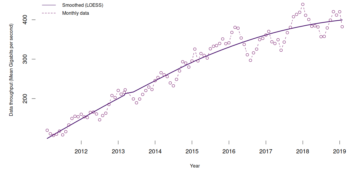
On a monthly scale, the data shows seasonal patterns, with increased internet traffic during the winter months and decreased traffic during the summer.
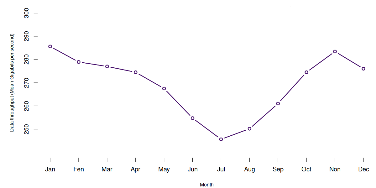
In Figure 2, monthly internet traffic since 2011 for a London Internet eXchange Point has been averaged which indicates a yearly parabolic pattern of use. Interestingly, this observation is the reverse of trends in UK road traffic reported in the DfT road traffic estimates. These show an increase in the number of cars passing a point during summer months, and a decrease during winter months.
If we consider purely leisure related internet use, the increase in traffic during winter months in this data may be due to reduced outdoor activity which may in turn be influenced by reduced daylight hours. If we consider “work” related internet use, the summer drop in traffic may also be further reduced by summer vacations and perhaps the aggregation of longer lunch time breaks during spells of good weather. In general, this month-by-month pattern is interesting in its own right, as it may be representative of general human seasonal activity.
Figure 2: LINX London average monthly data throughput, 2011 to 2019
Looking at daily internet traffic, many interesting patterns emerge. Figure 3 shows daily (London) traffic levels from the IXP data for 2016 and 2017 (most recent data at the time of the analysis) respectively. Each row corresponds to the day of week and each column corresponds to one of the 52 weeks in a year. Each cell represents the average internet use for each day in each week for the respective year – with bright cells representing higher internet use.
This visualisation shows that weekdays are different from weekends and that internet traffic tends to be lower in the summer months. It is also clear that certain days exhibit significantly less traffic volume.
Figure 3: Daily traffic levels from London IXP data, 2016 and 2017
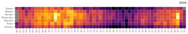
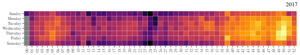
Figure 4 shows two years of internet traffic data for the London IXP. The vertical axis shows the relative intensity of traffic throughout the day, starting at 12am (bottom of the chart), through to 11:59pm (top of chart). Each point on the horizontal axis corresponds to one of the of 730 days in a period covering 2016 to 2017.
The dark band at the bottom of the visualisation corresponds to the morning hours between 2am and 7am, while the thin vertical dark bands correspond to lower internet traffic during the weekends. Although we use the internet at weekends and for leisure, we clearly use it more during the working week.
Figure 4: London IXP internet traffic data, 2016 to 2017

If we focus on April to May 2017, shown in Figure 5, three bank holidays are visible as three-day bands of lower traffic volume:
- Friday 14 April (Good Friday) to 17 April (Easter Monday)
- Monday 1 May (Early May bank holiday)
- Monday 29 May (Spring bank holiday)
While not surprising, the fact that the internet traffic throughput in this data varies according to work and non-work-days is an indication that the data may be useful for measuring working patterns and anomalous events.
Figure 5: London (LON2) IXP internet traffic data, April to May 2017

High frequency characteristics
During the average week, weekends tend to have lower traffic volumes, while mid-week days show the highest volumes of traffic.
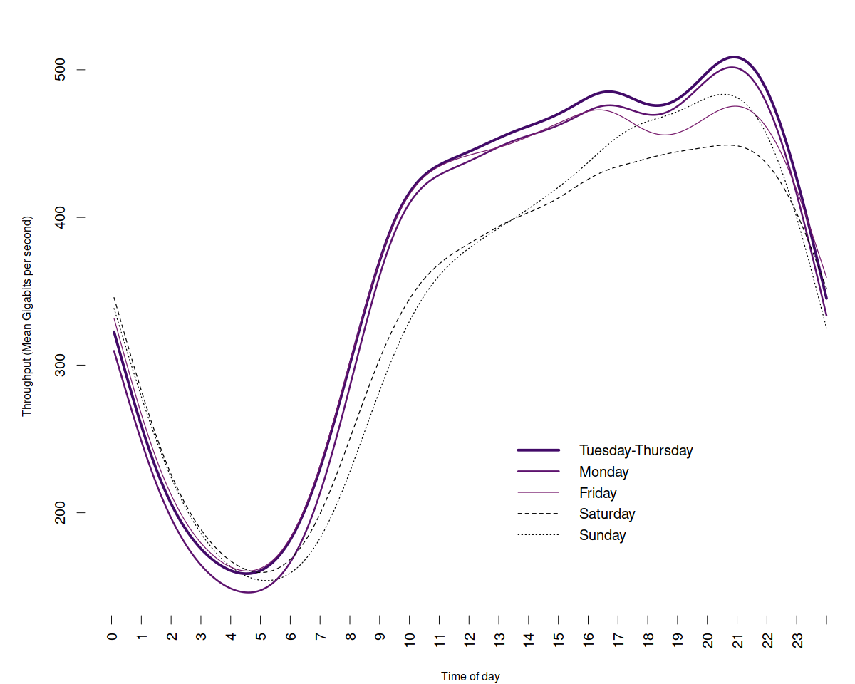
Some of the more interesting features of the data are the differences between the traffic volumes for each hour of each day of the week. Figure 6 shows the average hourly London IXP (LON2) usage in Gigabits per second (Gbps) for different times each day.
The weekdays follow a similar pattern, with each low point occurring at approximately 4:30am, followed by a sharp rise toward 10am. From 10am, traffic rises at a slower rate toward approximately 4:30pm. It then drops off until around 6pm before rising again to a daily peak at 9pm. In other words, although we are using the internet throughout the day, the heaviest use is during the working day.
An interesting feature is the difference between Fridays and the rest of the working week. Friday internet traffic tends to drop sooner, at a faster rate, and tends to be lower during the 6pm low point. This could be due to a tendency for people to finish work earlier on a Friday and to be more likely engaged in non-internet related leisure during the evening.
For all weekdays, there is a temporary drop in internet use which seems to reach a minima at approximately 6pm each day. This is one of the most notable characteristics and could be for several reasons, discussed later.
The average weekend usage is distinct from the weekday pattern. Besides being somewhat lower, Saturday and Sunday differ due to the missing 6pm dip. This could be due to a change in commuting activity during the weekend period. The 6pm dip during the weekday may be due to large-scale post work commuting behavior, where traffic volume (and generation) may change due to absence of use (for example, when driving a vehicle), a change in usage pattern while using mobile data, or change to an ISP which is not connected to the IXP.
In addition, Saturday and Sunday converge at approximately 1pm, at which point, Sunday’s (dotted line) usage tends to approach weekday evening peak use, while Saturday evening forms the lowest evening use in comparison to the rest of the week. Like Friday evening, it may be that the lower usage on a Saturday evening is due to increased (non-internet) leisure activity which defaults to the inter-week evening pattern on Sunday due to the next day being a work-day.
Figure 6: LINX London (LON2) average (5-minute) throughput per day
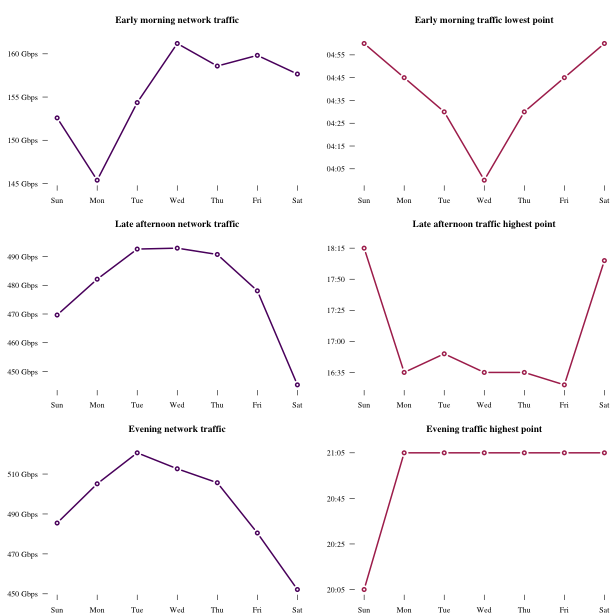
In addition to differences in the average daily traffic volume, there are also differences in the timing and extent of extremes during different time periods. Figure 7 shows the daily difference for traffic volume (left column) and low/high point time (right column) for the early morning low point (first row), late afternoon high point (second row), and finally, the evening peak (third row).
Starting with the early morning low point shown in the first row, we can see that, on average, Monday morning at 4:45am has the lowest internet use in our London sample data. As we move to mid-week, the early morning traffic volume increases, peaking on Wednesday before gradually declining toward the weekend. Interestingly, the time at which this low point occurs is symmetrically earliest mid-week (4am) and latest at the beginning and end of the week, where traffic is lowest at 4:45am on average.
The next notable feature is the extent and timing of the late afternoon peak which occurs just before the 6pm temporary drop in traffic each day. On average, the observed volume at this point is highest mid-week, inline with the overall average daily traffic and starting from Tuesday, occurs earlier each day toward the weekend. We speculate that this point delimits the end of the average working day and beginning of the daily commuting period.
Finally, the highest traffic levels can be observed each day at 9pm, with the exception of Sunday, where this peak time occurs one hour earlier on average. While the overall average daily internet traffic is highest on Wednesday, the evening volume is highest on Tuesdays.
Figure 7: Daily differences for traffic volume
4. Internet time use
In the previous section, we explored some of the high level characteristics of the data. In this section we explore the possibility that this data may be used to identify large-scale internet usage behaviour. Specifically, we examine the relationship between the data and results from a time-use survey and then explore the possibility that this data may be used to measure various aspects of day-to-day work and leisure phases.
2014-2015 time use survey
The Centre for Time Use Research 2014-2015 time use survey was a UK-wide survey which aimed to create a dataset describing how people spend their time throughout different days of the week. The survey was in the form of a user-kept diary which detailed specific activities for intervals of time.
Figure 8a shows the average amount of internet traffic for all 5-minute time points in a week for a London IXP (LON2), with the mean daily value shown by the orange dashed line. The inter-day variation could be explained by several factors. It is interesting to note that this variation is also present in the reported working hours in the time-use survey, as shown in Figure 8b.
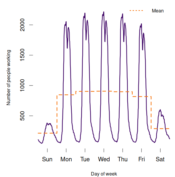
In the time-use survey, 3,523 participants logged their work status over a 7-day period in 15-minute intervals. By aggregating this data by day of week, we can see that Wednesday is the busiest day of the week, with Monday and Friday being significantly lower. Sunday is the least busy day (as expected). Comparing with the internet traffic data shown in Figure 8a, Wednesday is the busiest, with lower internet use at the weekends. This observation points in the direction that the internet use data may be influenced by economic activity (in this case, worked hours), and may also be of interest as an alternative (high-frequency) complimentary way to measure (internet related) time use.
Figure 8a: Average weekly data throughput
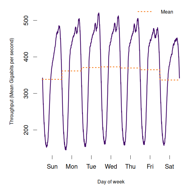
Figure 8b: Time-use survey work week
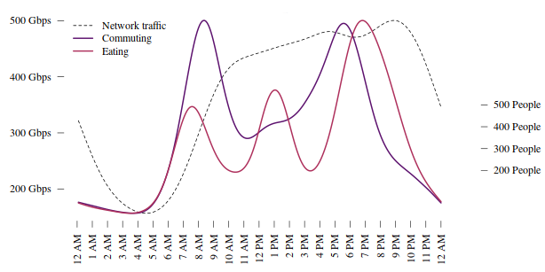
In addition to work time use, the time-use survey also includes a wide range of other activities. Figure 9 compares average daily internet traffic (dashed line) with number of people reporting to be commuting or eating for each point in the day. Commuting leads internet traffic use in the early hours of the morning (as expected). At 9am, as reported commuting activity declines the rate of change in internet traffic slows, and by 11am, both internet traffic and commuting activity begin to climb toward the 4:30pm late afternoon peak. Commuting activity proceeded by eating activity seems to account for the 6pm temporary low point.
Figure 9: Network traffic vs eating and commuting (2016 to 2017)
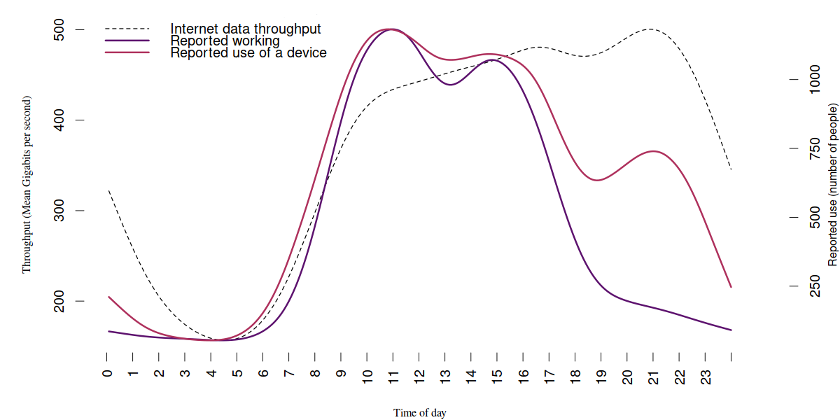
The time use survey contains an option to indicate use of a device (in combination) with other activities. The definition of a device includes use of a computer and as such, this reported activity appears to be highly similar to the average internet use. In Figure 10, we overlay the average number of people reporting to be working at each point in the day along with reported device use. Note that the 2014-2015 survey is from a different time period with respect to our data which extends into 2018, although it is interesting to note the similarity between the two series. The time and rate of change in internet use appears to coincide with working and device use during the morning hours. In addition, the 6pm drop and 9pm peak are inline with reported device use.
Figure 10: Average daily internet data vs time-use survey
Phase detection
As described previously, the average internet-day (in this data) can be divided up into various points in time and these points in time tend to vary, on-average, throughout the week.
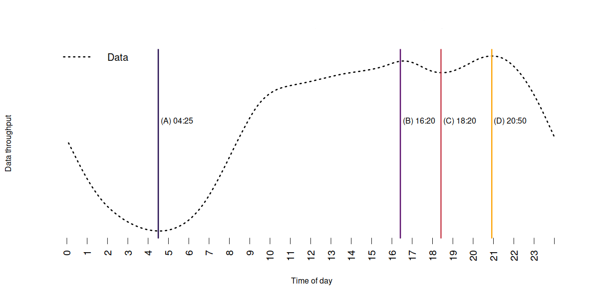
Specifically, these points correspond to the peaks and troughs which occur daily as shown in Figure 11.
In order to detect these points, it is first necessary to smooth the data. To do this, we fit a spline to each 24-hour period (it is also possible to use LOESS regression) and then attempt to identify the 4 sequential high/low points in each 24 hour period.
Having smoothed each day, we identify a change-point as the point at which the sign of the first difference changes. In combination with smoothing, this method is reliable in consistently identifying the 4 points of interest.
Figure 11: Data throughput changepoints (Average weekday)
As noted previously, the time at which these points occur varies through time as shown in Figure 12. In addition to varying throughout the week, interestingly the change-points also vary on average throughout the year.
Figure 12: Change-point variations by time of day
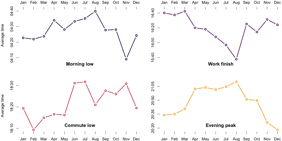
Figure 13 shows how the detected change-points vary on average through the year. The time at which the morning low (A) occurs is earliest in November where it tends to occur at 4:05am, steadily rising to 4:35am by August the following year. The point which we believe to mark the end of the working day (B) is one of the most interesting. It varies by approximately 1 hour throughout the year, being at its latest in the winter months (4:40pm), falling to its earliest point by August (3:35pm). The third point (C) marks the temporary low which occurs after the end of the work day. This could be related to commuting behaviour since it only occurs in weekdays. The final point (D), marks the so called internet rush hour which varies depending on the time-zone. Interestingly, this point occurs latest in the summer months, peaking at 9:05pm in August and occurs as early as 8:15pm in the winter.
Figure 13: Average change-point variation throughout the year
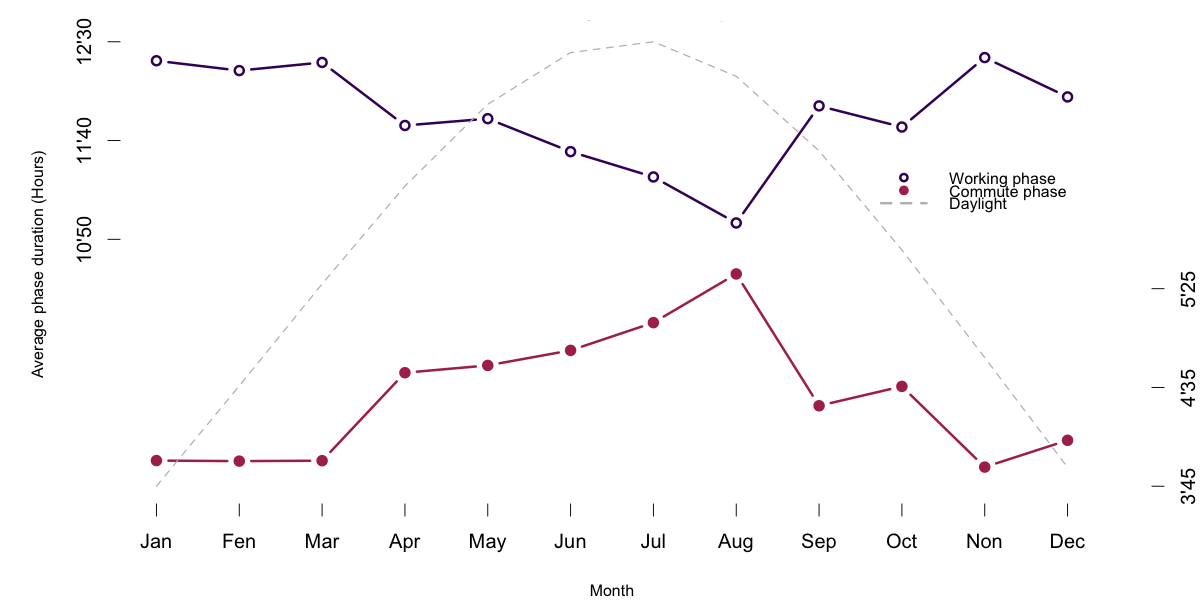
Based on change-points A,B and D, we have derived 2 indicators which measure the length of the “internet working day” (work phase – Figure 14a) and length of commuting period (commute phase – Figure 14b) which we define as the difference in time between points (A,B) and (B,D) respectively. The average monthly difference for each of the indicators is shown in Figures 14a and 14b. Both exhibit clear monthly seasonality, with the length of the internet working day being shortest in the summer and the length of the post work commute period being shortest in the winter months. We speculate that this monthly seasonality is due to the availability of daylight hours and road traffic conditions: road traffic tends to be higher in the summer, which may account for the length of the commute period.
Figure 14a: Internet traffic work and leisure/commute phase length
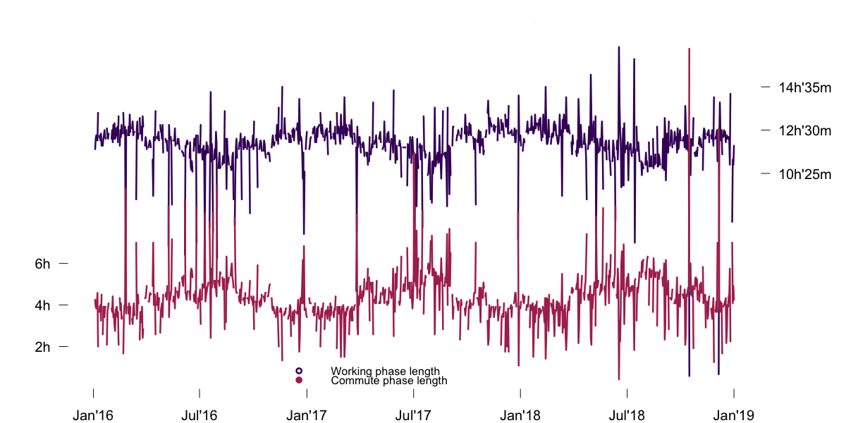
Figure 14b: Internet traffic work and commute phase length
5. Detecting anomalies and large-scale events
Using Singular Spectrum Analysis, we separate time-series into additive trend and periodic components which when added together, form a model \( m \) of the time series \( t \). The residuals, or noise, can then be defined as \( t – m \). This is the unexplained/anomalous part of the time series not captured by the model. These residuals can then be used to identify anomalies in the time series which may correspond to large scale events. Here, we show how the extent of these residuals relate to significant events.
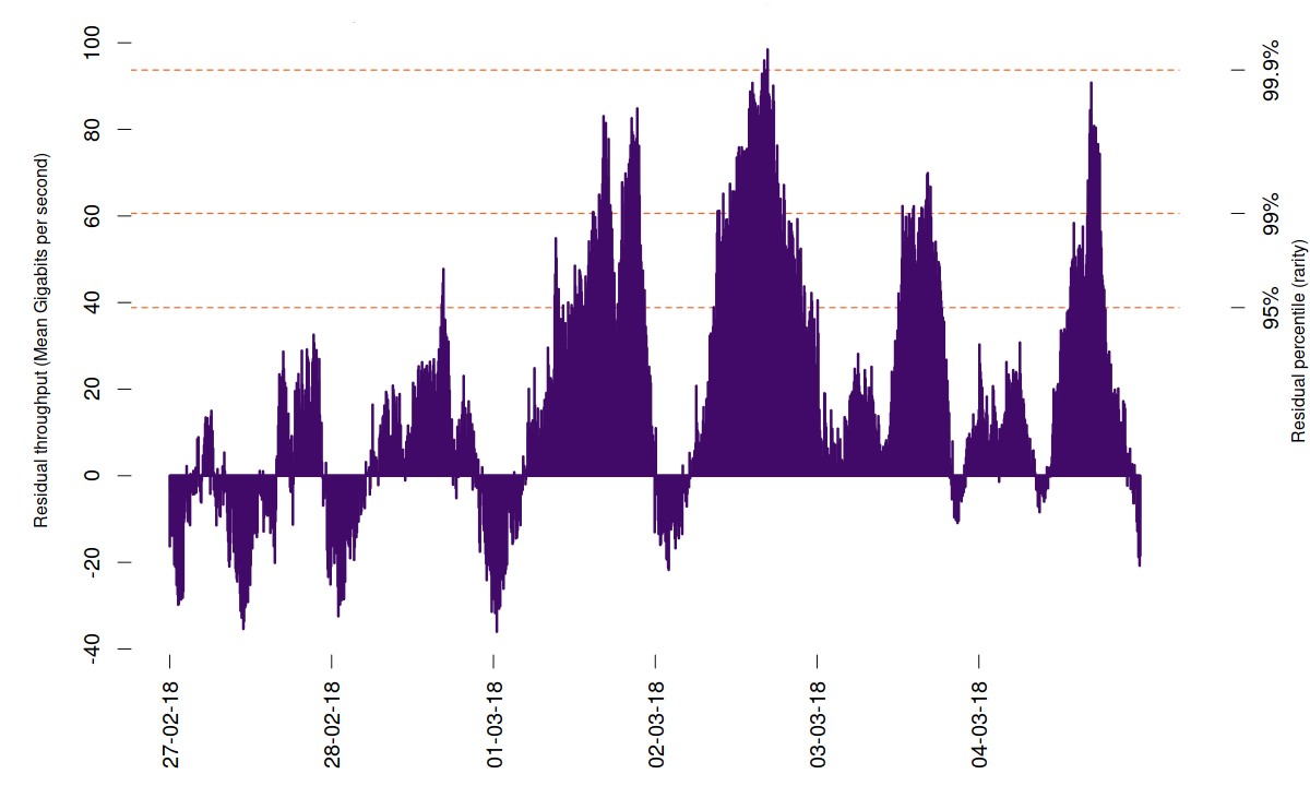
In the first example, we have been able to identify the effects of a significant weather event in the internet traffic data. At the beginning of 2018, there was a prolonged period of cold dubbed the “Beast from the East”. During this period of time, a winter storm named Storm Emma produced a significant amount of snowfall.
Figure 15 shows two days (A) and (B) where heavy snow fell on London. The result on the internet traffic data for the London IXP was a substantial increase in traffic which far exceeded the predicted level.
Figure 15: The effect of significant weather events on internet traffic data
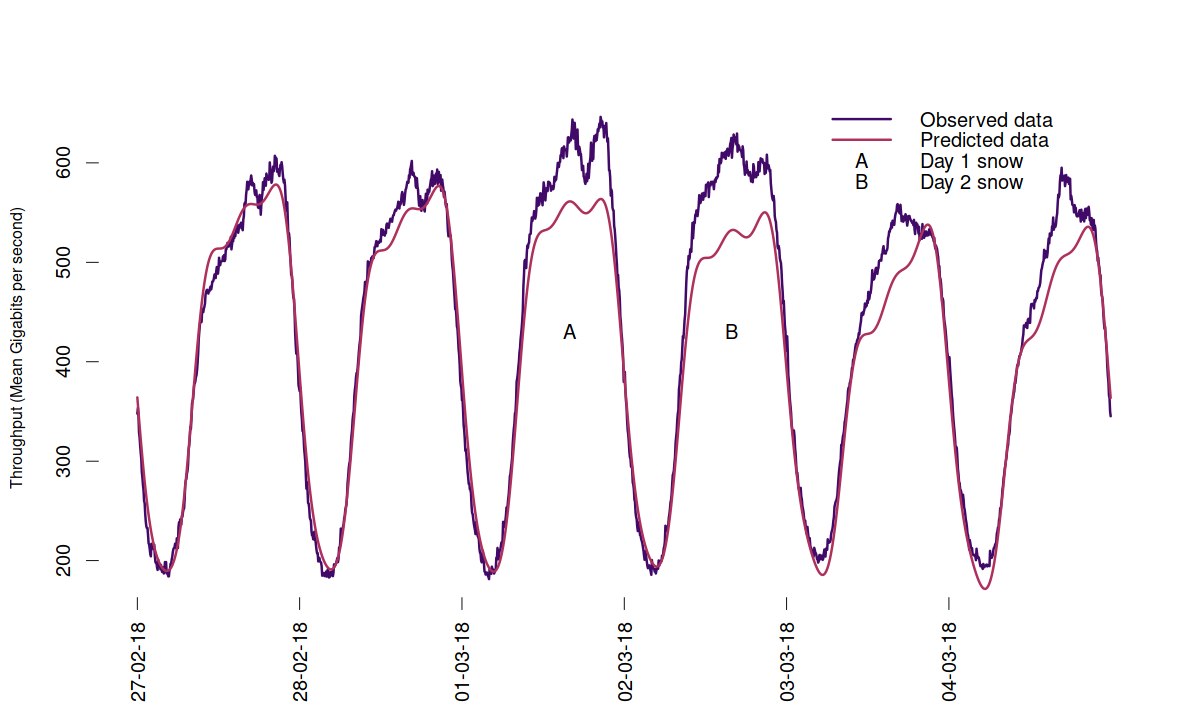
Figure 16 shows the resulting model residuals for the same period. The unexpected internet traffic on the second day of snowfall was at one point nearly 100 Gigabits per second (~ +20%) higher than anticipated. This increase in traffic could be due to an increase in people working remotely during the heavy snow and may also be due to people checking traffic updates or streaming video content.
In order to understand the significance of the event, we obtain the quantiles for each residual with respect to all residuals in our 2016-2018 dataset. In this example, the residuals are significantly higher (99 – 99.9 percentile) than all other observations.
Figure 16: Model residuals from Storm Emma and the Beast from the East
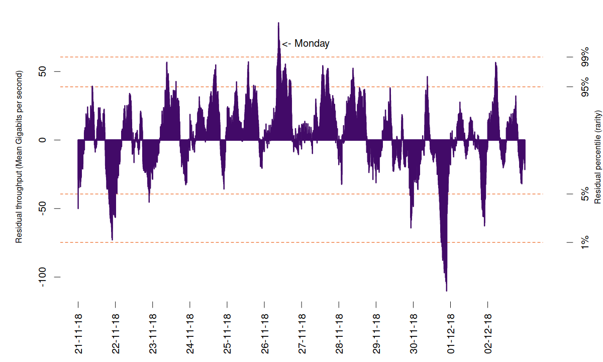
We next attempted to identify a significant retail event (Cyber Monday). In Figure 17 we show the most recent event from 2018 in which a spike in activity, above the 99% threshold occurs on Cyber Monday.
Although there is indeed a high residual on this day, it should be noted that it is short lived and resides within a range of other (significant) residuals during the same period. As such, it is difficult to assign any (speculative) meaning to this observation. Furthermore, we have been unable to identify such an effect in the previous 2 years.
Figure 17: Cyber Monday residuals, 2018
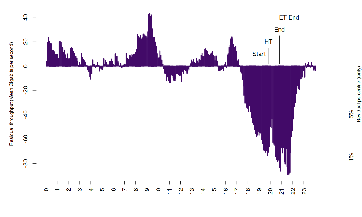
In the next example, we looked to identify a significant sporting event in the data. It is well known that football world cup games, given their large-scale audience, can impact internet traffic data. Figure 18 shows the extent of model residuals during the England vs Croatia men’s football world cup semi-final.
In this case, the event had a significant negative impact on traffic throughout the game. What is most interesting is that it possible to observe certain characteristics of the event. Specifically, the half time period and subsequent break in extra-time periods are clearly visible as temporary increases in traffic. In other games (not shown here), an opposite effect occurs in which traffic is substantially higher during the game and drops-off during half-time. This is likely due to the type of broadcast media. Some events may not be streamed, and people may be more likely to watch some events in pubs.
Figure 18: Football World Cup, England vs Croatia, 11 July 2018 residuals
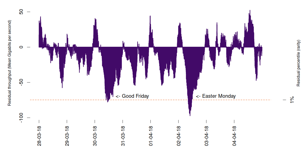
By far the most significant (sustained) exceptional events are bank holidays which have a -7.8% negative impact on average. In Figures 19a and 19b, the effect of the Christmas and Easter holidays are clearly visible in the form of a substantial decrease in traffic over each respective period. The Christmas period is particularly interesting as the effect covers a long period of time. On average, boxing day tends to have the most significant impact, with a -16% drop in traffic levels on average.
Figure 19a: Christmas period, 2017, residuals
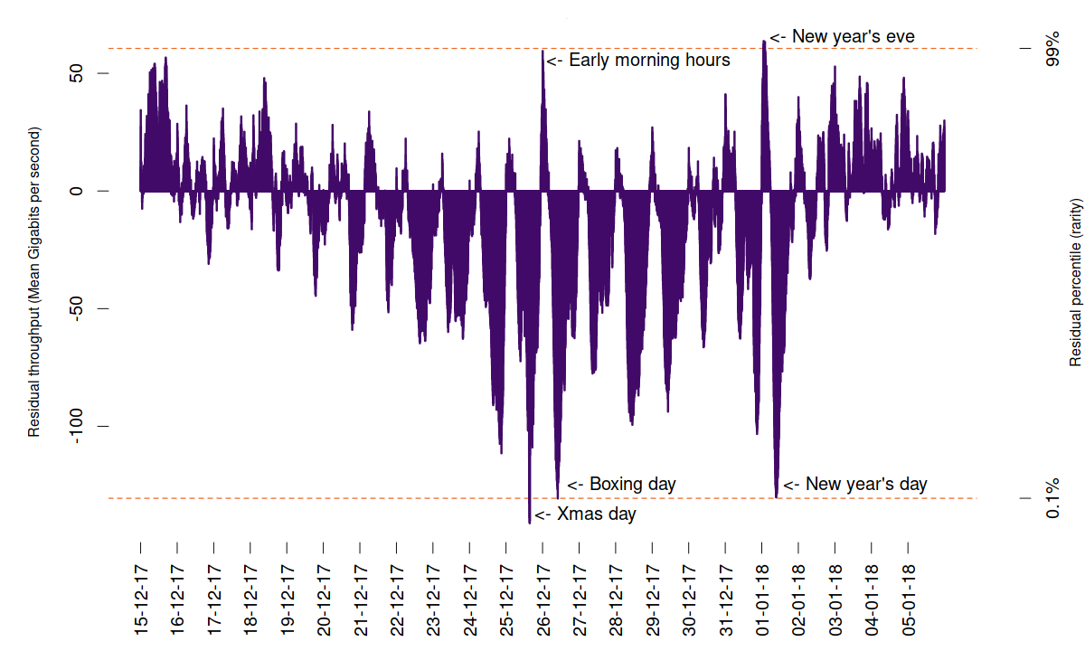
Figure 19b: Easter period, 2018, residuals
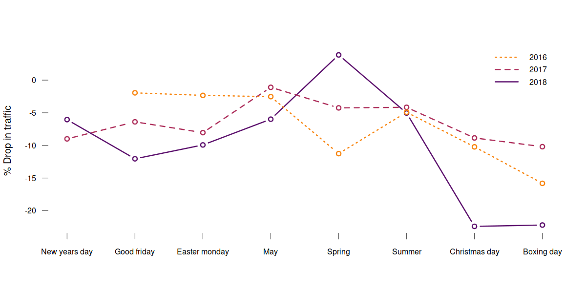
The extent of bank holiday impact appears to depend on the bank holiday as shown in Figure 20. These resulting observations are of interest since the average residual during each bank holiday period could be indicative of work force participation.
The previous examples show that various forms of large-scale events can be observed in the internet traffic data. This is of interest, since events of this scale may have some form of economic impact and measuring the extent over time may be of use as a potential proxy for the scale of impact. In addition to the events highlighted above, we have also been able to identify significant news events.
Figure 20: The effect of Bank Holidays on internet traffic
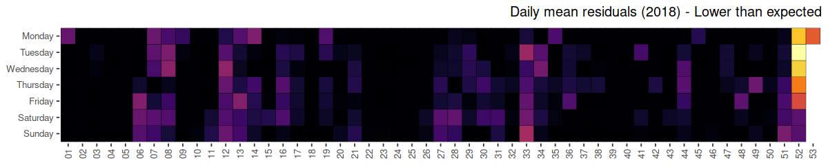
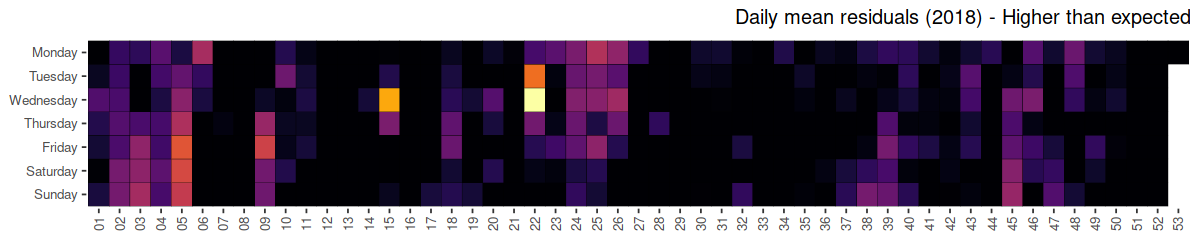
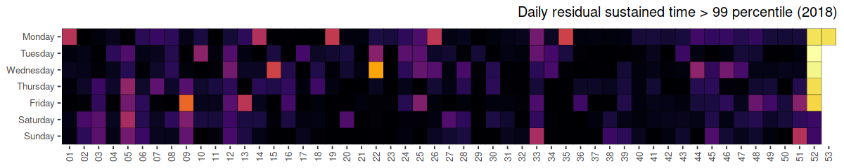
While we have highlighted a handful of events above, traffic anomalies with respect to our model residual occur frequently. Figure 21 demonstrates the presence of traffic anomalies throughout 2018. In the top row, we can see days in lighter colours in which at some point the traffic was significantly lower than anticipated, whereas the second row shows days in lighter colours where the traffic was significantly higher. In the final row, we show days where the internet traffic was consistently significant through each day: brighter points indicate days where the traffic was above or below the 99% significance level for a long period of time.
Figure 21: Traffic anomalies, 2018
6. Relationship with economic activity
Our exploratory analysis of a novel data source has highlighted the potential value for internet traffic volume data, and has pointed to some valuable areas for future research. One such area is the relationship between this data and existing economic indicators. Initial analysis of the relationship between the IXP internet traffic use and monthly Gross Value Added (GVA) suggests that the data may be correlated with specific sectors of the economy during specific time periods. This is a challenging direction of research since we might expect little relationship with components of GDP given that GDP does not measure certain aspects of internet activity. Also the data at present does not allow us to split the component of internet traffic related to work as opposed to leisure.
The work also points to the potential for producing a range of derivative indicators. For example, we noted before the difference in Friday evening internet activity compared with the rest of the week. It may be possible to use the extent of this difference as a proxy for evening (non-internet related) social activity which may in turn be used in the context of understanding the night time economy.
7. Relationship with road traffic data
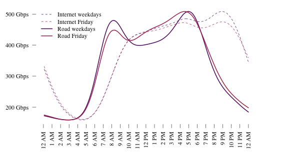
This exploratory research has also highlighted the possibility that the IXP internet traffic data could be used to indirectly measure road traffic, and more generally, commuting behavior.
This idea is based on the observation that the 4-6pm drop in internet traffic coincides with the commuting period. If we can measure the depth, breadth and timing of this temporary drop in internet traffic, we expect to find a relationship with average road traffic speeds and public transport use.
Figure 22 shows the relationship with UK-wide average weekday road traffic reported as an index of average car miles in the Department for Transport’s Road traffic estimates compared with (London) IXP internet traffic data. The reported road traffic data are in line with the results from the time-use survey and furthermore exhibit similar characteristics to the internet traffic data. On Fridays in particular, there is an overall increase in road traffic data coupled with a decrease in internet use data.
To date we have explored road traffic count data from the M25 motorway surrounding London. We have found that the monthly seasonality of the data exhibits a negative relationship, in that internet traffic tends to be lower in the summer months whilst road traffic tends to be higher.
Figure 22: Average weekday road traffic index (car miles), and London IXP data
8. Conclusion
We have described an interesting and novel data source, internet traffic volume data, which we are using as a step in the direction to explore scalable methods for measuring data-driven social-economic activity. The purpose of this post has been to discuss some of our observations and initial ideas and to describe the direction of our current research in this area. We have touched on the possibility of using this type of data to estimate components of time-use surveys, specifically, we have derived a set of internet-day length indicators which vary depending on the day of week and throughout the year. We then demonstrated how large-scale social events manifest in this data in the form of anomalous data consumption, we believe this has the potential to yield insights into large-scale events such as adverse weather conditions and sporting events.
In addition to time-use and large-scale events, our analysis has pointed to some valuable areas for future research, including the relationship between internet traffic data and various established economic indicators, and the relationship between internet traffic and road traffic. As a novel line of investigation, we believe there to be a relationship between the post 4pm dip in internet traffic and peak time road traffic for the geographical area around an IXP. The implication of such a relationship would be a scalable proxy measure for city commuting behaviour which binds the virtual and physical world. Such a proxy measure could be applied globally.
9. Acknowledgements
This work has benefited greatly from discussions and feedback from the LINX community. We give special thanks to Kurtis Lindqvist for his help and invaluable feedback during this project.
We would also like to thank colleagues from Economic Statistics at the ONS, and the Economic Experts Working Group for their contributions to this work.