Using data science to explore changes in behaviour and well-being during the coronavirus (COVID-19) pandemic

The coronavirus (COVID-19) has had a massive impact on the UK economy and population. In the months since the initial lockdown began in March 2020, daily behaviour has changed significantly as the population adapts to the steps taken to curb the spread of the virus. The importance of identifying these changes is critical to both government and industry.
In this blog, we outline how machine and deep learning may be used to explore changes in population behaviour during the coronavirus pandemic using the 2015 and 2020 Time Use Survey (TUS) data. We introduce:
- an interactive tool to rapidly and efficiently explore the TUS data, identifying specific regions of interest that may be investigated in greater detail by additional analysis
- a novel, data-driven framework to identify pre-COVID-19 working time and well-being-based behaviours, using factors including paid or unpaid work, childcare, commuting and those based upon the 5 ways to well-being
- a means to explore behavioural changes during the initial national lockdown; this can measure impact upon both the high-level population and much smaller and more focused cohorts of individuals such as those based upon age, family and retirement
- an approach to measure and predict well-being based upon activity enjoyment, providing a link that allows us to explore the less tangible impact of the pandemic upon well-being at an individual level
- a technique to track well-being changes in the population during COVID-19
- an approach to simulate the link between policy and well-being that can be used in either a reactive (what is the effect) or proactive (what will the effect be) way to estimate the impact of policy changes upon well-being within the population
Applied in isolation, these techniques are insightful and informative. In combination, they provide a broad toolkit that allows us to better explore and quantify the impact of the coronavirus upon the UK population in terms of both work-based behaviour and well-being.
1. Data
The United Kingdom Time Use Survey (UKTUS) was a UK-wide 2014 to 2015 survey that captured how people spend their time in every 10-minute period over a 24-hour window. Verbatim responses were coded into one of 278 possible activities relating to areas such as employment, childcare, leisure, housework, shopping, travel, and so on. Before each individual completed the survey they were interviewed, and household and individual level data were captured including demographic, employment, education, and health. Approximately 9,300 individuals were surveyed, each producing up to two diary days of activity resulting in over 16,500 days of activity available for analysis in the leisure time in the UK study.
The 2020 Online Time Use Survey (OTUS) is based upon UKTUS with a specific focus upon digital activities, the sharing economy, equalities and well-being. 1,200 individuals took part in the survey, producing over 2,000 diary days of data relating to 66 activities. The initial survey was completed in March and April 2020 during the first national lockdown with additional waves planned across 2020. As the time gap between the 2015 and 2020 surveys is significant and sample sizes are limited, caution must be exercised in assigning cause to effect. To that end, this report focuses more on discussing possible analytic approaches rather than concentrating on the results themselves. Any results we present, although based upon real data, should be treated as exploratory rather than definitive.
Consequently, this report is not intended to replace current work at the Office for National Statistics relating to the analysis of the Time Use Surveys and national well-being (links to this work are given throughout this report).
As with many surveys, the Data Science Campus faced a significant challenge relating to data volumes. This limited not only our ability to focus on specific cohorts within the population (such as those defined by affluency, ethnicity, disability), but also in the choice of machine and deep learning techniques applied to the data.
Interactive visualisation tool
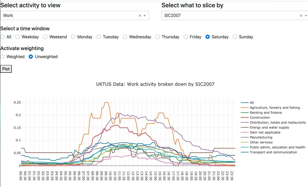
To quickly explore the large volumes of survey data, an interactive visualisation tool was developed in Python using Dash. This presents the proportion of the population undertaking an activity across the day the survey was completed. The resulting distributions can be presented at population level, broken down by the data collected in the pre-survey interviews, reweighted to match the wider population (using sampling weights) and broken down by the day of the week. Figure 1 shows the proportion of the population working on Saturday, broken down by Standard Industrial Classification 2007 (SIC). It is clear to see that the greatest proportion of people working are those within the agriculture, hotels and restaurants, and constructions industries. Not unsurprisingly, the working patterns relating to hotel and restaurant workers are skewed to later in the day and into the evening.
This example illustrates how we may rapidly explore the behaviour space and extract high-level insight relating to population behaviour at a point in time and (by comparing between UKTUS and OTUS surveys) across time. This identifies areas where additional analytic effort may be focused.
Figure 1: Proportion of population in each SIC2007 code working on Saturday
2. Exploring working time and well-being behaviour
To further explore the differences in behaviour between the 2015 and 2020 surveys, we firstly simplify the complexity of the behavioural space. We reduce the number of time slots from 144 to 96 by only considering activity between 0700 and 2300; this minimises the likelihood of “sleeping” dominating the analysis.
We minimise the number of possible activities by aggregating into higher-level representations, consistent across both surveys. The “working time” aggregate activity classifications and a representative set of the lower-level classifications are shown in Table 1.
Table 1: Aggregate working activity classifications
| Not working | None of the other groups |
| Paid work | Main paid work
Part-time paid work Lunch break Coffee break |
| Unpaid work | Household chores
Gardening and DIY Food shopping Helping other adults Voluntary work |
| Childcare | Feeding
Teaching Reading to Accompanying |
| Commuting | Travelling to and from work
Travelling for work |
The “well-being” aggregate activities were based upon the 5 ways to well-being, with additional sleeping and timeout categories added (Table 2).
Table 2: Well-being activity classifications
| Sleeping | |
| Timeout | Reading
Listening to music Watching TV |
| Connection | Contact with people and pets |
| Active | Exercise and activity |
| Learning | Class-based
Self-learning Homework |
| Awareness | In bed not asleep
Resting |
| Helping | Volunteering
Teaching Helping adults and children |
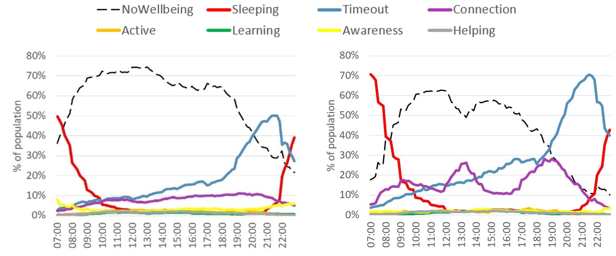
Figure 2 shows the reweighted distributions of aggregated activities before and during the early stages of the coronavirus pandemic. Each line gives the proportion of the population undertaking that aggregate activity across the day. There are some obvious and expected differences between the two samples. For “working time”, there is an increase in unpaid work, an increase in childcare and a reduction in commuting, both before and after the working day. In the case of well-being (Figure 3), there is an increase in the proportion of the population sleeping later into the morning. Connection during lunchtime and after work has increased with a sizeable increase in timeout across the evening. These findings are generally consistent with those found in the weekly Opinions and Lifestyles Survey.
Figure 2: (Left) Population level working time behaviour 2015 (benchmark); (Right) Population level working time behaviour March / April 2020
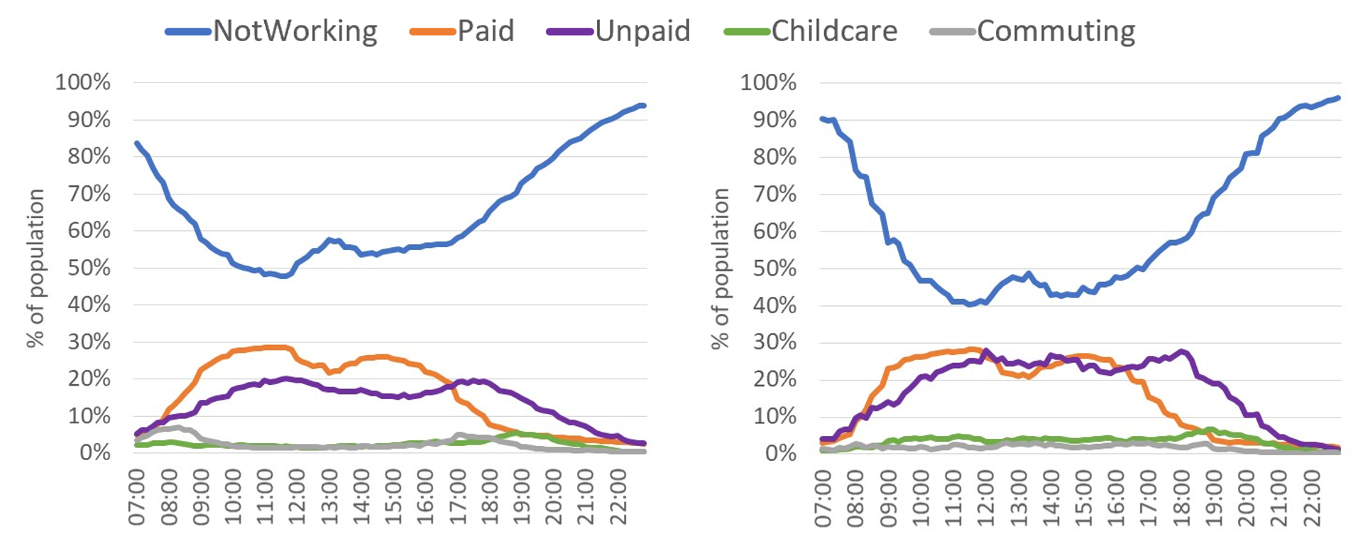
Figure 3: (Left) Well-being behaviour 2015 (benchmark); (Right) Well-being behaviour March and April 2020
The behavioural frameworks
Although informative, comparing behaviours at a population level provides only a high-level view, with more subtle behaviours being missed. We address this by segmenting the benchmark sample to discover unique working time and well-being-based behaviours within the population. These behavioural frameworks are then applied to the 2020 survey data, and the changes in segment membership across the population compared.
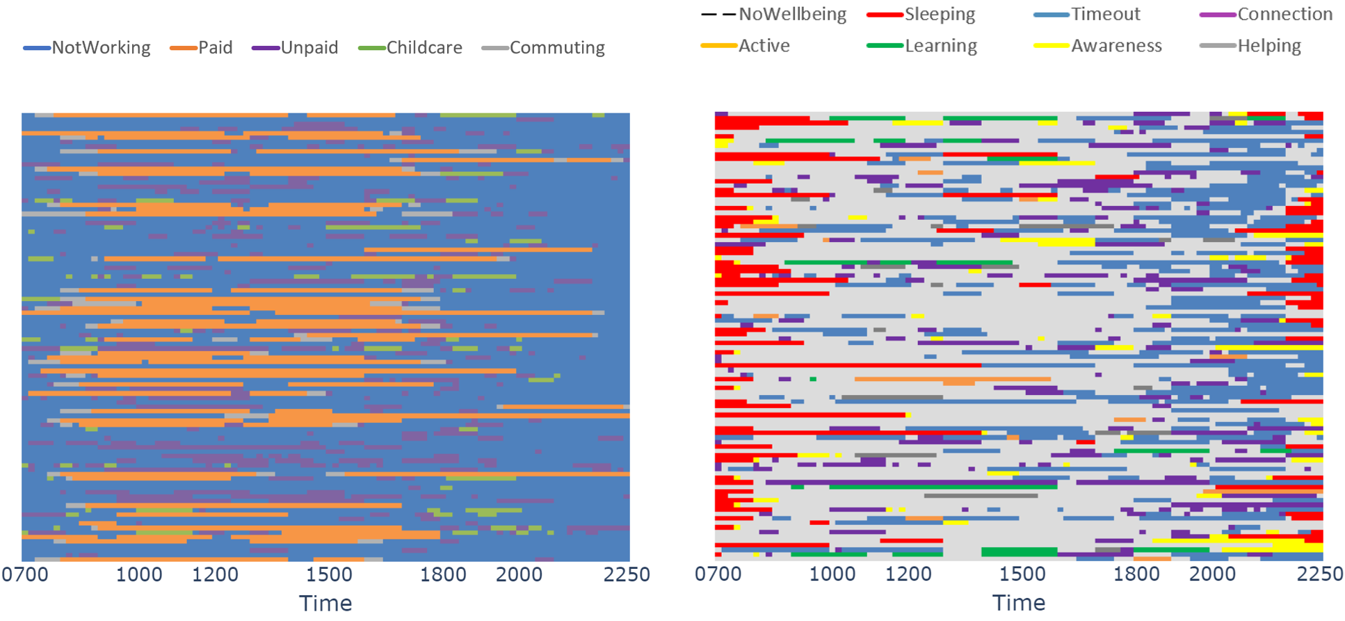
Because of the complexity of the behavioural space (Figure 4), it is impractical to manually define the segments. We use unsupervised kmodes segmentation, where the survey response for every individual is encoded a vector with each element representing one of the aggregate activities for a given time slot.
Figure 4: (Left) Aggregated working time activity for 50 randomly chosen individuals; (Right) Aggregated well-being activity for 50 randomly chosen individuals
The training sample is reweighted to match the wider population using weights with the datasets. Overlay variables including age, gender, location, job type and household composition are used to profile and contextualise each segment. To ensure each segment related to population behaviours, overlay variables were not used to segment the population.
Seven working time segments were generated (Table 3).
Table 3: The working time segments
| 1 x Non-working | Non-working |
| 3 x Paid | Day workers
Early workers Late workers |
| 3 x Unpaid | Morning peak
Lunch time peak Afternoon peak |
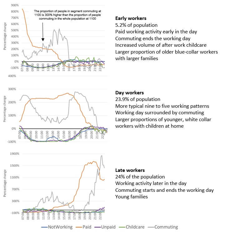
Figure 5 introduces the profiles for three of the seven segments, relating to paid work. These are:
- early workers corresponding to 5.2% of the population
- day workers corresponding to 23.9% of the population
- late workers corresponding to 24% of the population
Of the remaining segments, the non-working segment is more likely to contain the older and younger members of the population, who are either in full-time education or retired. The final three unpaid segments relate to peaks of unpaid work in the morning, lunchtime and afternoon, with comparatively large volumes of childcare predominantly undertaken by females.
Figure 5: The “paid” working time segments (each line represents the proportion of people in that segment undertaking that aggregated activity, expressed relative to the whole population)
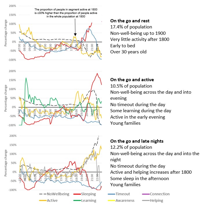
Eight well-being segments were generated (Table 4). The profiles of the three On the Go (OTG) segments are shown in Figure 6 and these are:
- On-the-go and rest corresponding to 17.4% of the population
- On-the-go and active corresponding to 10.5% of the population
- On-the-go and late nights corresponding to 12.2% of the population
Individuals in these segments are time-pressured to undertake well-being-based activities across the day. The main difference between these segments is how spare time is utilised. This is either relaxing for “OTG and rest”, learning, exercise and activities for the “OTG and active” or limited well-being for the “OTG and late night” segment.
Table 4: The well-being segments
| 1 x Relaxed | Chillout |
| 2 x Learning | Late start students
Easy days and learning |
| 2 x Helpers | Daytime help and relax
All day help |
| 3 x On-the-go (OTG) | OTG and rest
OTG and active OTG and late nights |
Turning to the remaining well-being segments, the relaxed segment contains significantly higher than average timeout activity across the day, generally relating to the older age groups. The first of the learning segments is late start students, where full-time students massively over-index for sleep into mid-afternoon and then learn into the night and beyond (for more information relating to the impact of COVID-19 upon students see Coronavirus and the impact on students in higher education in England: September to December 2020). The second learning segment contains much older individuals who also learn during the day but start and finish earlier with a period of timeout in the evening. Finally, the two helper segments relate to helping activity across the day. Individuals in the daytime help and relax segment over-index for over 50-year-old males; their helping activity drops significantly in the evening and is replaced by timeout. All-day helpers are made up of much younger individuals with families. Their help not only covers the daytime, but is extended into the evening, with a smaller period of timeout much later in the day.
Figure 6: The “On the Go (OTG)” well-being segments (each line represents the proportion of people in that segment undertaking that aggregated activity, expressed relative to the whole population)
Applying the frameworks
Armed with this data-driven framework, we allocate every individual surveyed during March and April 2020 to one of the segments generated from the 2015 UKTUS data. This allows us to explore behaviour changes during the first national lockdown of the coronavirus pandemic.
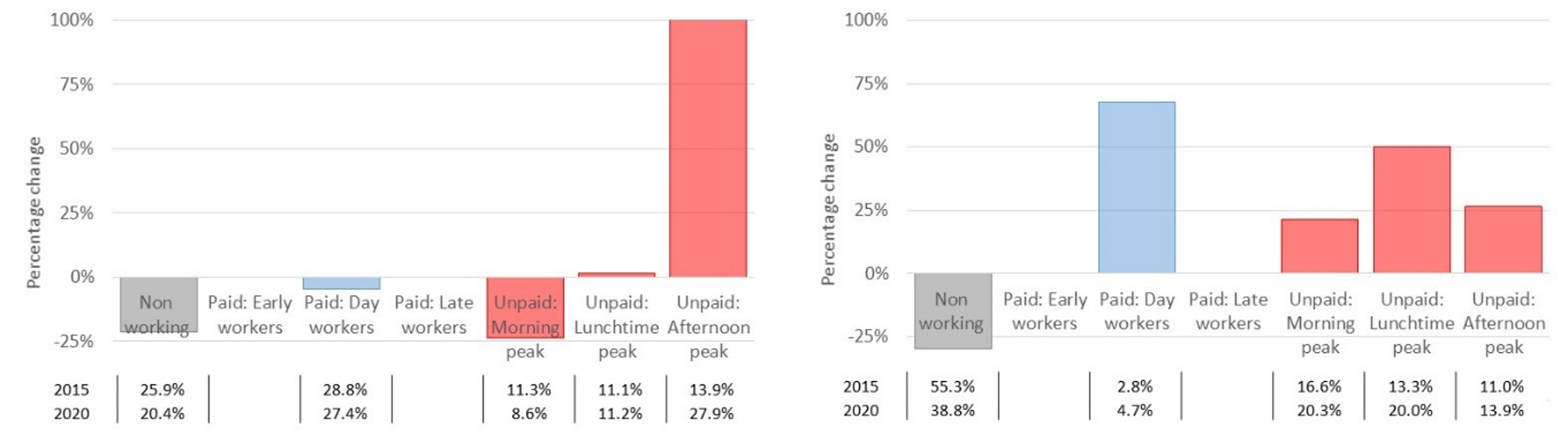
The charts in Figure 7 give the proportion of the base falling into each segment. Each bar gives the percentage change for the 2020 figures expressed relative to the 2015 figure.
Figure 7: (Left) Working time segment changes; (Right) Well-being segment changes. March and April 2020 population distribution indexed against 2015
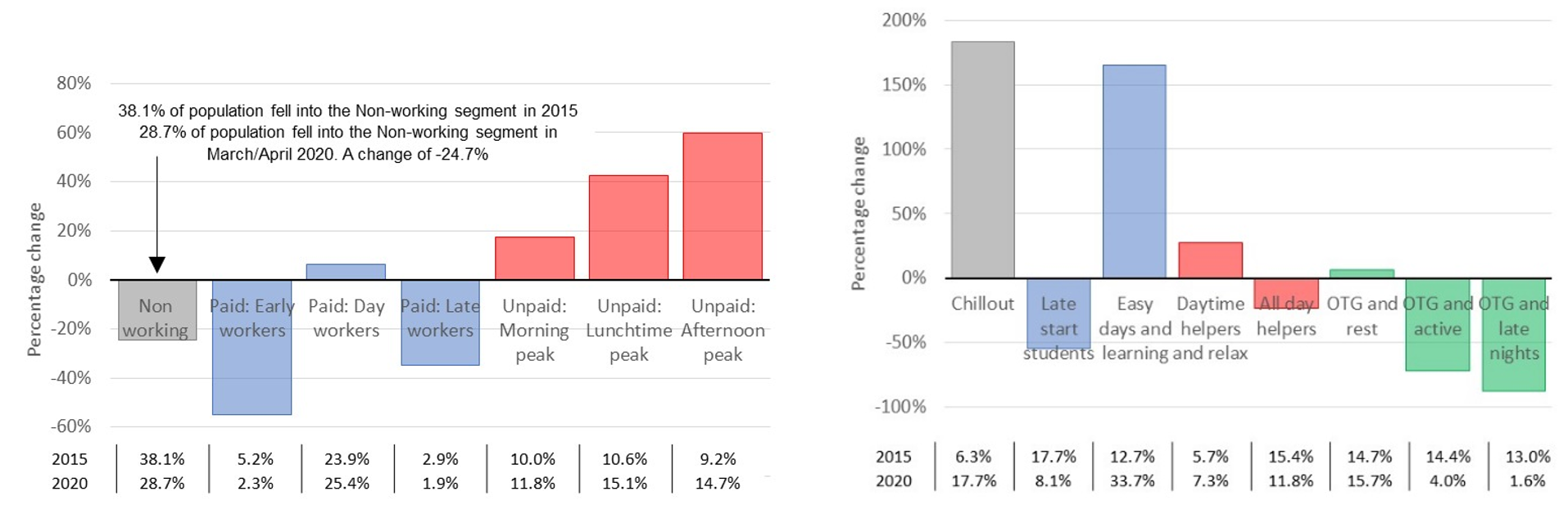
For the working time behaviours, there are significant increases in the number of people falling into all three unpaid segments, possibly caused by the closure of schools, the reduction of childcare provision and the furlough of paid workers. Both early and late paid workers have decreased, caused in part by the inability of many blue-collar workers to work from home. Paid day workers have increased slightly, suggesting a degree of migration into this segment by other paid workers who are able to work from home.
The changes in the well-being segmentation are greater in magnitude, significantly in the “chillout” and “easy days and learning” segments. This reflects the increase in furlough-related spare time. All three OTG segments have reduced, notably in the most active and family-oriented “OTG and active” and “OTG and late nights” segments. This may reflect the fact that parents furloughed or working from home are under less time pressure with regards to childcare and domestic chores. Finally, the reduction in late start students is indicative of the closure of schools and universities.
A very powerful application of the behavioural segment framework is to track the classification of individuals over time. Unfortunately, there is no way to link individuals across surveys, as it is very unlikely that individuals surveyed in 2015 were also surveyed in 2020. So instead, we track cohorts of individuals over time. Initially we compare March and April 2020 against 2015, but additional waves will provide a longer-term view of behavioural changes.
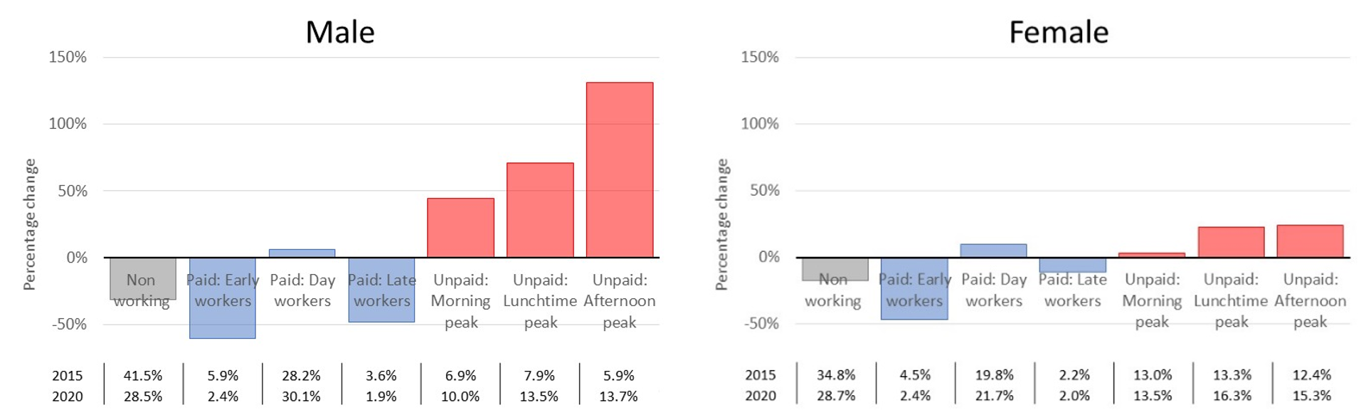
Figure 8 shows working time behavioural changes for the male and female cohorts. Migration from the paid to unpaid segments is more evident in the male cohort. Smaller movements for the female cohort reflects the fact that they are already disproportionately responsible for childcare and household upkeep, with male unpaid time more likely to be spent doing activities such as DIY and gardening.
Figure 8: Working time segment changes, broken down by gender, male (left) and female (right). March and April 2020 population distribution indexed against 2015
Turning to the young families cohort (left on Figure 9), the most significant increase is within the unpaid afternoon peak segment, supporting research that suggests that parents working from home delivered most childcare in the afternoon. Looking at the retirement age cohort (right on Figure 9), a reduction in the non-working segment and an increase across all three unpaid segments may be because of an increase in gardening and DIY-based activities.
Figure 9: (Left) Working time segment changes for the households with young children cohort; (Right) Working time segment changes for the retirement age cohort
3. Exploring the link between enjoyment and well-being
COVID-19 has impacted upon well-being and depression within the population, see Coronavirus and depression in adults, Great Britain: January to March 2021. The approach discussed above can easily be expanded to use the well-being segment framework to explore this impact. However, this only indicates changes in the behaviours that are known to affect well-being, it does not indicate if the individuals have higher or lower levels of well-being, nor if behaviour changes during the coronavirus (COVID-19) pandemic are beneficial or detrimental from a well-being standpoint.
In both the 2015 and 2020 Time Use Surveys (TUS), the participants were asked to score each activity based upon their enjoyment of it. Research by the Office for National Statistics (ONS) and wider research community suggests that the link between happiness and well-being is a strong and measurable one. Additional work suggests that enjoyment of both work and leisure activities also have a significant impact upon well-being. Applying these findings, we use the enjoyment score as a proxy for well-being.
Unfortunately, differences in the survey design make direct comparison across surveys problematic. Although both surveys asked the individual to assign an enjoyment score from one (not at all) to seven (very much), the 2020 survey explicitly specified level four as being a “neutral” response. Consequently, certain activities, such as sleeping, are more likely to receive a neutral score in the 2020 survey. As a result, although the data presented in Figure 10 were taken from the surveys, it is only intended to demonstrate how these data may be used. It should be treated as illustrative and not definitive, with no insight drawn from it.
Figure 10 gives the percentage change in enjoyment score broken down by well-being segment (rows) and aggregated well-being activity (columns).
Figure 10: Enjoyment changes across segment/activity group (OTG, On the Go) Because of survey differences, results of this chart should be treated with caution
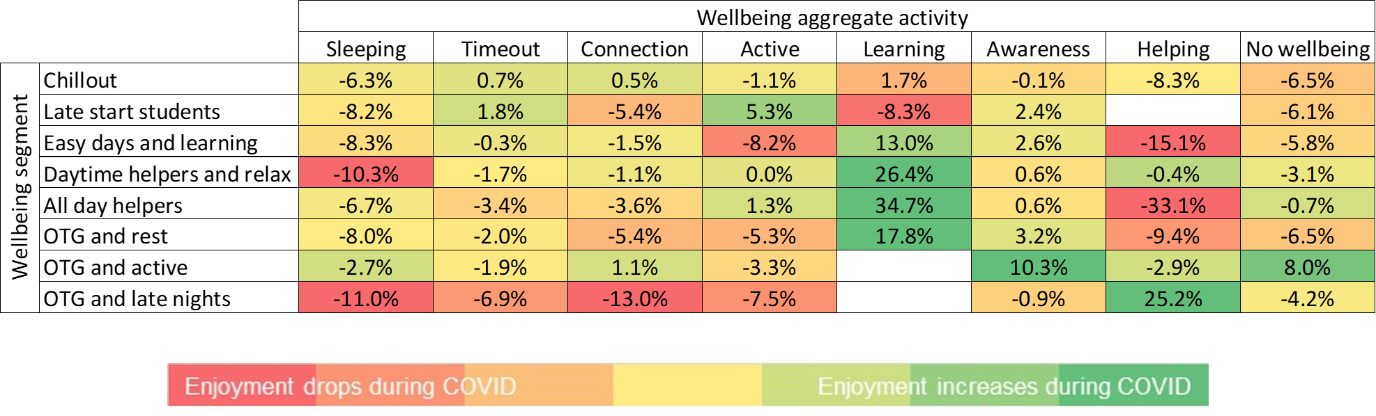
This chart can be used to explore several things. Each column gives an indication of how the enjoyment of a specific activity changed during the first national lockdown for each segment, and therefore the sensitivity of each activity. For example, the enjoyment of learning has increased within most segments, decreasing only for the late start students’ segment. Conversely, the enjoyment of helping has decreased for all but one of the segments.
Each row represents the impact of the coronavirus pandemic upon the individuals in each segment. Segments with the greatest overall reduction in enjoyment are interpreted as being more affected from a well-being perspective. Individuals within the on the go (OTG) and late-night segment appear to be more sensitive than individuals within chillout or OTG and active segments. We may also identify the activities that may be driving this sensitivity, with enjoyment of connection-based activities for individuals in the OTG and late-night segment being particularly significant.
Predicting activity enjoyment
As survey data are limited, the resulting sparsity makes it challenging to understand the dynamics of enjoyment at an individual level. The relationship between features is generally not consistent between individuals. For instance, the enjoyment of education is generally far lower for a child where education is compulsory, when compared with an older age adult who has chosen to learn.
We propose a supervised approach to capture these complex relationships and to interpolate within sparse regions of the feature space. Ideally, we would predict change in enjoyment as presented in Figure 10. However, for reasons discussed earlier, enjoyment data cannot easily be compared across surveys. Instead, we focus on predicting activity enjoyment during the initial lockdown phase of the coronavirus pandemic.
We use certain factors to strike a balance between predictive power and parsimony. These are:
- enjoyment of preceding activities in the last hour (autoregressive features)
- previous activities undertaken in the last hour
- time of day and day of week of activity
- an individual’s age, gender, country of residence, working time and well-being segment
- number of adults, children, and young children in household
We found that using autoregressive data beyond the preceding hour added little performance improvement and increased model complexity considerably. To eliminate sparsity when encoding the 66 categorical activities into one hot encoding space, we instead used an approach based on word embedding. Here, the activities were “embedded” into a much lower number of floating-point values (see Cat2Vec) with two embedded values giving optimal results.
Three model approaches were investigated. These were:
- naive model
- non-recurrent XGBoost
- recurrent stacked LSTM deep neural network
The naive model is a simple look-back-one model with the current enjoyment predicted as being the enjoyment of the previous activity. The XGBoost and Long Short Term Memory (LSTM) models are more sophisticated techniques using the features to predict a multi-class output with each output class relating to one of the seven enjoyment levels.
Within the XGBoost model, the activity embeddings were generated independently using a standalone embedding based neural network. In the LSTM model, an embedding layer was incorporated directly into the network architecture and optimised during training. All other categorical features were converted to one-hot encodings. A randomised grid search was used to tune the hyperparameters and network architectures. Validation and test datasets were used to avoid overtraining and to assess performance.
Table 5 gives model performance. The most striking finding being the high overall accuracy achieved by the naive model. We are forced to deploy very sophisticated machine and deep learning techniques to improve upon it. This illustrates the importance of the autoregressive inputs in a temporal model such as this, as they capture the general happiness of the individual. If we look across each enjoyment class, we can see that the naïve model performs relative poorly in the low enjoyment classes. This is likely caused by the lack of data in these classes and the temporal isolation of low enjoyment activities (if you are doing something you do not enjoy, you are more likely to stop and do something you do).
Table 5: Test dataset results – XGBoost and LSTM models including autoregressive features
| Enjoyment | Naive Precision | Naive Recall | XGBoost Precision | XGBoost Recall | Stacked LSTM Precision | Stacked LSTM Recall |
| 1 (low) | 0.869 | 0.872 | 0.959 | 0.839 | 0.950 | 0.879 |
| 2 | 0.867 | 0.866 | 0.930 | 0.862 | 0.968 | 0.903 |
| 3 | 0.876 | 0.876 | 0.935 | 0.881 | 0.935 | 0.901 |
| 4 | 0.922 | 0.924 | 0.927 | 0.937 | 0.950 | 0.955 |
| 5 | 0.915 | 0.914 | 0.922 | 0.918 | 0.947 | 0.935 |
| 6 | 0.932 | 0.931 | 0.931 | 0.942 | 0.940 | 0.957 |
| 7 (high) | 0.955 | 0.955 | 0.961 | 0.958 | 0.970 | 0.968 |
| Accuracy | 0.931 | 0.937 | 0.952 | |||
As you would expect, the more sophisticated XGBoost and LSTM models using richer input features are better equipped to overcome these issues and outperform the naive model both in overall accuracy and precision/recall within each class. However, these models still rely predominantly upon the autoregressive inputs. In the case of the XGBoost, 28 of the 30 most powerful features relate to the autoregression of activity enjoyment.
Although these models are useful from a predictive standpoint, the dominance of the autoregressive features masks the more subtle drivers of low enjoyment and well-being. To address this, models were built without the autoregressive inputs. As expected, the accuracy of both models drops (Table 6). However, performance approaching 70% for a seven-class problem, where random accuracy would be 14%, is still impressive.
Table 6: Test dataset results – XGBoost and LSTM models excluding autoregressive features
| Enjoyment | XGBoost Precision | XGBoost Recall | Stacked LSTM Precision | Stacked LSTM Recall |
| 1 (low) | 0.905 | 0.553 | 0.701 | 0.543 |
| 2 | 0.930 | 0.551 | 0.669 | 0.497 |
| 3 | 0.868 | 0.462 | 0.568 | 0.546 |
| 4 | 0.695 | 0.644 | 0.714 | 0.675 |
| 5 | 0.702 | 0.587 | 0.637 | 0.639 |
| 6 | 0.662 | 0.703 | 0.659 | 0.669 |
| 7 (high) | 0.688 | 0.813 | 0.743 | 0.772 |
| Accuracy | 0.690 | 0.687 | ||
The relative importance of XGBoost features are shown in Table 7. This can be interpreted as being the features that have the greatest effect (positive or negative) upon well-being in the context of the model. It is reassuring that the two most important features relate to the activity itself. The emergence of both working time and well-being segments in the list is a further example of the power of the behavioural framework introduced earlier.
Table 7: Top 15 non-autoregressive features (XGBoost)
| Feature | Relative importance |
| Activity embedding dimension 1 | 0.0316 |
| Activity embedding dimension 2 | 0.0240 |
| Age | 0.0235 |
| Working segment: Paid early workers | 0.0203 |
| Working segment: Paid day workers | 0.0195 |
| Two children in household | 0.0189 |
| Live in England | 0.0188 |
| Live in Wales | 0.0188 |
| Well-being segment: Late start students | 0.0187 |
| Two or more young children in household | 0.0187 |
| Well-being segment: OTG and rest | 0.0187 |
| Female | 0.0184 |
| Well-being segment: OTG and active | 0.0184 |
| Activity falls on a Monday | 0.0180 |
| Activity falls on a Wednesday | 0.0177 |
Applying the activity models
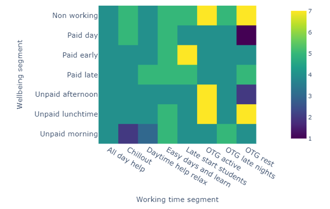
Using the LSTM model, well-being at an individual level is explored by generating enjoyment geometries. Here, the values of a subset of features are fixed, with the remaining features being systematically sampled and enjoyment predicted in each case. For ease of interpretation, we generate 2D planes, however this approach can be applied to any number of features, resulting in an n-dimension hypercube. Figure 11 shows the working time and well-being enjoyment plane for a middle-aged man with a young family when washing up on Monday evening. Here, we can see that the enjoyment varies widely across the slice, with values ranging from high enjoyment when the individual falls into the OTG and active/not working segments, to the low enjoyment with the OTG and rest/paid day segment.
Figure 11: Well-being and working time segment enjoyment plane for a middle-aged male living with his partner and two children, when washing up on Monday evening (1 lowest enjoyment, 7 highest enjoyment)
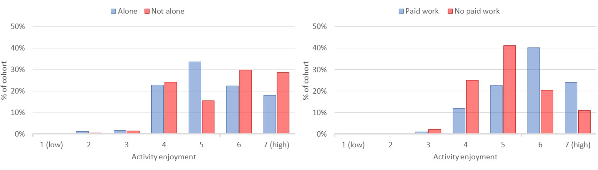
Finally, we explore how changes in personal circumstances may have an impact on the well-being of an individual. To do this, we run two simulations: with and without the changes. In each simulation, the model predicts the enjoyment of a random activity undertaken at a random time on a random day. This is repeated 100,000 times to get a representative view of the enjoyment across all activities for that individual. Predicted enjoyment values for each simulation are then combined to provide an overall enjoyment distribution. The difference between these distributions reflects the changes in well-being of the individual.
Figure 12 (left), shows the impact of living alone for a 70-year-old male compared with living with another adult in the household. Figure 12 (right) shows the impact of unemployment for a 25-year-old male who lives with his partner and two young children. The enjoyment of everyday activities and, therefore, overall well-being has notably reduced for both the 70-year-old man if he lives alone and for the man with family responsibilities, should he lose his job.
Figure 12: (Left) Impact of living alone for a 70-year-old male; (Right) Impact of unemployment upon a 25-year-old male with a young family
With enough data producing a more performant model, both of these approaches can be used to simulate the impact of policy upon well-being. Policy changes that may alter the personal circumstances of an individual, the behavioural segments they fall into or the mix of activities they undertake across the day, can be used to predict the changes in activity enjoyment of that individual. These changes can be aggregated to population level and used in either a reactive (what is the effect) or proactive (what will the effect be) way. This will help to gain insight into the impact upon well-being of that actual or proposed policy change.
4. Summary
In this report we have outlined how machine and deep learning may be used to explore changes in both working and well-being behaviour during the early stages of the coronavirus (COVID-19) pandemic using the 2015 and 2020 Time Usage Survey (TUS) data. A number of novel and powerful techniques were introduced, and examples given in each case. These approaches covered many of the main analysis steps from initial data exploration using a Python-based interactive visualisation tool indicating specific areas of interest and utility within the TUS data through to a deep learning model that, can be reactively or proactively used to simulate the link between policy and the well-being at both individual and population level.
From a machine and deep learning perspective, where datasets with tens of thousands of training records or larger are the norm, the comparatively small sample sizes in the TUS data limits the robustness and confidence that may be placed upon the presented results at this time. Consequently, all results, although based upon real data, are illustrative rather than definitive and no actionable insight should be drawn from them.
Bearing this caveat in mind, it is pleasing that the results presented in this report consistently support the findings of more statistically robust work undertaken by the ONS. It is therefore suggested that with larger data samples or data taken from additional waves throughout and beyond the coronavirus pandemic, the techniques outlined in this blog would provide a powerful and robust toolkit that would allow us to better explore and understand the impact of the coronavirus upon the UK population in terms of work-based behaviour and well-being.