Technical report: nowcasting UK household income using the new “signature” method

Economic nowcasting refers to generating estimates of the current (“now”) state of the economy. It involves using advanced time series methods to combine information released at a high frequency (indicators) to estimate what a lower-frequency variable of interest (target) might be doing in real-time.
In this technical report, we generate nowcasts from a range of different methods for quarterly UK household income using a set of within-quarter information (with different publication lags) that are available at a higher frequency than the current quarterly household income estimates. This research has been useful for the household income team at the Office for National Statistics (ONS), as they seek the best methods to generate estimates so decision makers can gain the best early indications about the state of the economy.
This report is part of a programme of work that the ONS has been doing with the Alan Turing Institute to explore the usefulness of various economic nowcasting methods, particularly the signature method. The signature method has been used previously in other disciplines like finance, healthcare, and cyber security. We have been investigating if it could also be useful for economic nowcasting. Other outputs from our work may also be of interest.
A paper details how the signature method compares against other nowcasting methods mathematically and in various empirical applications, including nowcasting US gross domestic product (GDP) and UK road fuel prices. There is also a PYTHON code repository which enables others to apply the signature method to generate nowcasts for other variables of interest.
The appetite for nowcasts arises because households, businesses, and policymakers want up-to-date information to make the best decisions. However, it takes time to collect and compile information that accurately represents the whole economy. Therefore , official estimates of key economic indicators are published with a delay. For example, the ONS currently publishes its first quarterly estimate of UK household income around six weeks after the end of the quarter it refers to.
However, there is a vast wealth of information about aspects of the economy that can be gleaned from data that are released more quickly and frequently. For instance, the UK is one of a small number of countries that publish GDP monthly estimates (based on output measures) and also publishes a weekly Economic activity and social change in the UK, real-time indicators bulletin. Others are available from other sources.
Nowcasts utilise these more frequently released indicators to infer what is happening to a particular variable of interest (for example, household income) in the economy now.
There are two challenges facing nowcasting. The first is the so called “ragged-edge” problem caused by missing values of different indicator variables at the end of the sample period because of different publication delays. The second is issues arising by use of mixed-frequency data, whereby some explanatory indicators are published at a higher-frequency than the variable of interest. An example would be a nowcast where the low-frequency target is published quarterly and the high-frequency explanatory indicators are published monthly.
There are a variety of nowcasting methods that handle these challenges in different ways. In this report, we consider three main methods:
-
- the bridge method
- the mixed-data sampling (MIDAS) method
- the signature method
In addition, we use an autoregressive model as a baseline comparator.
We examine how nowcasts generated using each of these methods perform empirically, compared against the first release of quarterly UK household income. We also examine the data chosen in the models to gain some understanding of what kind of data could be useful to explain and nowcast household income.
We find that nowcasting household income is challenging. We find that the MIDAS method offers a slight improvement over the autoregressive baseline and one potential advantage is that it captures some of the movement in the household income realisations, whereas the autoregressive model is a broadly constant nowcast which may be less useful in informing decision making.
Other methods, including the signature method, produce similar performance to the autoregressive baseline and there is limited improvement when more indicators become available. This may be because the explanatory power of the set of indicators we have explored is limited and varies over time.
The report proceeds by describing the data used in our models in Data and the methods used to compute the nowcasts and select the variables in Methodology. We present the nowcasts and the variables that are selected in Empirical results before concluding.
Table of contents
1. Data
The household income data we use as our target variable is quarterly growth in our Compensation of Employees time series. It measures the total renumeration, including wages, salaries, and supplements to wages and salary, earned by employees in return for their work done during an accounting period. According to our UK Economic Accounts time series, compensation of employees made up about 50% of gross domestic product (GDP) in 2022.
We identify a set of real-time monthly indicators that could be informative about our target. Table 1 provides information about the set of monthly indicator variables and the target we consider. The first and the second columns give their name and the acronym or codes we use in this report. The third column shows whether the variable is of quarterly (Q) or monthly (M) frequency.
The set of indicators we use include sources used in the compilation of Compensation of Employees statistics gathered from the Office for National Statistics (ONS). These include Average Weekly Earnings (AWE) and two variables from the Labour Force Survey (LFS):total actual hours (TTH) and gross weekly pay (GRSSWK).
Since household income is a large component of GDP, we also investigate variables that have been considered in GDP nowcasting literature. In particular, we make use of the dataset produced by Anesti, Galvão and Miranda-Agrippino’s nowcasting paper (2020) (PDF, 821KB. We select from their dataset the real-time data series of Retail Sale Index (RSI), Index of Production (IOP), Index of Services (IOS), and Manufacturing Production (MPROD). As their real-time dataset contains data up to the last quarter of 2018, we update the real-time vintages using data from the ONS to cover the whole of 2019.
As in Anesti, Galvão and Miranda-Agrippino’s nowcasting paper (2020) (PDF, 821KB), we also include Mortgage Approval (MTGAPP), Net Consumer Credit (NCC), and Agent Score (AS) in our set of indicators. We also collect the most recent data series directly from the Bank of England. These are static series, and their past values are not revised. The Agent Score series we use is Total Business Services. In addition, our set of indicators include Claimant Count (BCJA) and Sterling Effective Exchange Rate (SEER) data from the ONS, the House Price Index (HPI) from HM Land Registry and the Consumer Confidence Index (CCI) of the UK from the OECD. Hence, the set of indicators we use for our analysis provides information about the following:
- household income components
- labour market condition
- production
- services and sales
- housing market
- credit and borrowing
- purchasing power
- general sentiment of confidence
Understanding the publication lags and timeliness of monthly indicators is crucial in nowcasting, as it determines which nowcast horizons should be considered. We establish three nowcast horizons: t+0 day, t+15 days and t+45 days where t denotes the end of the reference quarter for which we generate a nowcast. The last three columns of Table 1 indicate how much in-quarter information is available for each monthly indicator variable.
Our first nowcast horizon (t+0 day) is at the end of the reference quarter, so for example, an estimate for UK household income in the first quarter of a year would be generated at the end of March. At this horizon, most of the monthly indicators we consider only have their first month estimates (within the reference quarter) available.
The next nowcast horizon we consider is 15 days after the end of the reference quarter, so for example, an estimate for UK household income in the first quarter of a year would be generated in mid-April.
Our last nowcast horizon (t+45 days) is 45 days after the end of the reference quarter, so for example, an estimate for UK household income in the first quarter of a year would be generated in mid-May. This horizon is designed to be equivalent to the timing of the first official estimate.
New information about the monthly indicators become available as one moves through the nowcast horizons because of publication lags. In Table 1, if we were to focus only on the indicator variable Index of Production (IOP), at nowcast horizon t+0 day, data has been published about the first month of reference quarter(month 1, m1). By nowcast horizon t+15 days, data for the second month of the reference quarter (month 2, m2) has been published and by nowcast horizon t+45 days, data is available about all three months of the reference quarter. As well as including the information for a new month, there may also be revisions to previous estimates.
The timeliest indicator is CCI, whereby the first nowcast horizon (t+0 day) there is already information about all three months within the reference quarter. By nowcast horizon t+15 days, we see from Table 1 that the estimates of all the real-time indicators for the second month have been published. The estimates of Claimant Count for the three months within the quarter are also available.
At nowcast horizon t+45 days, we have estimates for all three months within the reference quarter for all variables. The only exception is that since August 2016 there is no longer an Agent Score (AS) produced for the third month of the reference quarter because of a change in the Monetary Policy Committee meeting schedule (see Bank of England’s Definitions for the Agents’ scores). Given that the most recent in-quarter dataset at this horizon is available for indicator variables, predictions are expected to be the most accurate. However, as nowcasts at this horizon are close to the publication of household income estimates for the reference quarter, the timeliness of the prediction may not be as useful.
For household income and most monthly indicators, we compute the percentage change between reference months. The exceptions are Agent Score (AS), where we use the values at levels, and Net Consumer Credit (NCC), where we scale the dataset according to the quartile range. Both variables already represent the change relative to the period before, so we have no need to use any transformation that would force this data to be stationary, such as the percentage change. The percentage change transformation is used to achieve stationarity and to help us nowcast the quarterly growth rate.
We nowcast the quarter-on-quarter growth of household income using the set of transformed indicator variables.
Table 1: The availability of monthly information across nowcast horizons
| Data | Acronym/Code | Frequency | t+0 days | t+15 days | t+45 days |
| Target variable: | |||||
| Household income | DTWM | Q | |||
| Monthly indicator variables: | |||||
| Consumer Confidence Index | CCI | M | m1, m2, m3 | m1, m2, m3 | m1, m2, m3 |
| Industrial Production | IOP | M | m1 | m1, m2 | m1, m2, m3 |
| Average Weekly Earnings | AWE | M | m1 | m1, m2 | m1, m2, m3 |
| LFS gross weekly pay | LFS_GRSSWK | M | m1 | m1, m2 | m1, m2, m3 |
| LFS total count hours | LFS_TTH | M | m1 | m1, m2 | m1, m2, m3 |
| Claimant Count | BCJA | M | m1, m2 | m1, m2, m3 | m1, m2, m3 |
| House price index | HPI | M | m1 | m1, m2 | m1, m2, m3 |
| Manufacturing Production | MPROD | M | m1 | m1, m2 | m1, m2, m3 |
| Index of Services | IOS | M | m1 | m1, m2 | m1, m2, m3 |
| Retail Sales Index | RSI | M | m1, m2 | m1, m2 | m1, m2, m3 |
| Mortgage approval | MTGAPP | M | m1, m2 | m1, m2 | m1, m2, m3 |
| Net Consumer Credit | NCC | M | m1, m2 | m1, m2 | m1, m2, m3 |
| Sterling Effective Exchange Rate | SEER | M | m1 | m1, m2 | m1, m2, m3 |
| Agent Score (Total Business Services) | AS | M | m1, m2, m3 | m1, m2, m3 | m1, m2, m3 |
Our estimation sample covers the period 2005 Quarter 1 (Jan to Mar) to 2014 Quarter 1, and the nowcast evaluation sample covers the period 2014 Quarter 2 (Apr to June) to 2019 Quarter 4 (Oct to Dec). There are 23 quarters in our evaluation sample. We produce recursive nowcasts of the first estimates of UK household income using the latest information available for the monthly indicator at the time when we need to produce a nowcast. It is worth noting that we omit the coronavirus (COVID-19) pandemic in our evaluation sample. It is because such an event may alter the relationships learnt by the models during the estimation sample. In the next section, we describe the set of models we use to nowcast UK household income.
2. Methodology
In order to nowcast UK household income, we employ nowcasting models that can accommodate mixed frequency data and handle missing data issues and are widely used in macroeconomic nowcasting literature. These models include the bridge method with Autoregressive Distributed Lag (ARDL) and the Mixed Data Sampling (MIDAS) model. We compare their empirical performance with the nowcasts produced using the signature methods. To benchmark these models, we implement an autoregressive model with one lag and a constant term as a comparison, detailed in section Autoregressive benchmark.
In this section, we give an overview of the nowcasting models we use. We also discuss how we arrive at a subset of indicators that are useful to explain household income as selected by shrinkage methods, and how we compute nowcast recursively throughout the nowcasts evaluation period.
Nowcasting models
The nowcasting methods used in our research overcome key challenges in nowcasting in different ways. These include the ragged-edge problem, where there may be missing data at the end of the time series because of publication lags, and the mixed frequency problem, where we are trying to predict a quarterly outcome using monthly explanatory indicators.
Bridge method
The bridge method overcomes these issues by taking a two-step regression approach to the nowcasting problem. In the first step, an autoregressive model is implemented to fill any missing values in the explanatory indicators (zt) that are present because of publication lags (1). When the dataset is complete, the high-frequency data is aggregated to the same time-period as the low-frequency outcome variable (2), in our case, from monthly to quarterly; if xt is a quarterly average of zt, then for all s we have γs = 1/3. The second step regresses the low-frequency target (yt) on the aggregated indicator variables (xt) alongside an autoregressive process in the target variable (3). \( \)
$$ z_{t} = \delta_{0} + \sum_{s=1}^{p} \delta_{s}z_{t-s}+\eta_{t} \ \ \ (1)
\\
x_{t} = \sum_{s=0}^{2} \gamma_{s}z_{t-s} \ \ \ (2)
\\
y_{t} = \sum_{s=1}^{p} \alpha_{s}y_{t-3s} + \beta_{0} + \beta_{1}x_{t} + \varepsilon_{t} \ \ \ (3) $$
MIDAS model
MIDAS is a method commonly used for nowcasting. MIDAS overcomes the mixed-frequency and ragged-edge problem by generating a single parameter for each high-frequency explanatory indicator, for each low-frequency outcome period, using the most recent indicator data and its lags available in that period. The parameter is generated using a polynomial lag function, which applies weights to the most recent value and its lags (see equation (5)). Once parameters have been generated to overcome dimensionality issues, a non-linear least squares model (4) can be applied to produce estimates for our outcome variable. In this piece of research, we apply an exponential almon lag, as shown in (6), to our data to generate the parameterised data.
$$ y_{t} = \sum_{s=1}^{p} \alpha_{s} y_{t-3s} + \beta_{0} + \beta_{1}x_{t} + \varepsilon_{t} \ \ \ (4)
\\
x_{t} = \sum_{s=0}^{p} \gamma(s, \theta) z_{t-s} \ \ \ (5)
\\
\gamma(s, \theta) = \frac{exp(\theta_{1}s + \theta_{2}s^{2})}{\sum_{j=0}^{p}exp(\theta_{1}j + \theta_{2}j^{2})} \ \ \ (6) $$
For a more detailed overview of both bridge and MIDAS nowcasting methods, see Schumacher’s discussion paper (2014) (PDF, 550KB).
Signature method
Signatures are mathematical objects (iterated integrals) of paths or continuous time series, which capture useful geometric information. It has universal approximation properties; linear regression on signature terms can describe any relationships between the indicators and the target variable, including nonlinear relationships. The path signature has an infinite number of terms, but because they are decreasing rapidly (at a rate faster than exponential) in size, we are theoretically justified to take a truncated form for practical purposes. This truncation typically occurs in “levels”, which is the number of integrals taken to compute the term. Each integral can be taken with respect to any of the indicator variables, so if there are d indicator variables, then there are dn signature terms at level n. We refer to the family of methods using truncated signatures in regression as the “signature method”.
While this method has been applied across other disciplines, it is largely unexplored in economics. The signature method handles the nowcasting challenges of missing and mixed frequency data by first embedding the observed data in continuous time through interpolation techniques. We then find the signature terms up to a specified truncation level and use these terms as explanatory variables in a linear regression to nowcast the target variable. \( \)
$$ Y_{t} = \sum_{k=0}^{K} (\alpha_{k} + \beta_{k}Y_{t-})\varphi_{k,t} + \varepsilon_{t} \ \ \ (7) $$
Where Yt is some prior observation of the low-frequency target at the point of nowcast. φk,t is a sequence (for each value of t) of signature terms at truncation level k, which includes the iterated integrals of t alongside components of the observed process X (for instance, the high-frequency observed explanatory variables), within some specified rolling window. αk and βk represent vectors of regression coefficients.
A more in-depth introduction of path signatures and its properties is given by Chevyrev and Kormilitzin in their Primer on the Signature Method (2016) (PDF, 1,183KB). To see further explanation of the signature method and its uses within the context of nowcasting, see the paper produced by this programme of work [LINK] (which also contains a more detailed explanation of bridge and MIDAS too).
Autoregressive benchmark
We benchmark nowcasts produced by these models against the forecasts of household income produced by an autoregressive model (AR). We examine the appropriate number of lags to be included in the AR model using the Akaike Information Criterion (AIC) and find that the first order autoregression, that is, AR(1), is most appropriate. Therefore, we use AR(1) forecasts as a benchmark to allow us to determine if within-quarter information is useful to predict the target.
Variables selection
Using a robust subset of information to improve model performance is a strategy widely adopted in macroeconomic analysis. Potential methods used for choosing a robust subset include model selection statistics (such as adjusted R2, Information Criteria, tests for individual or joint significance of variables), stepwise selection methods and shrinkage methods. These methods are well-established in the time series literature and widely used in empirical analysis for finding an informative set of indicators to explain the variable of interest.
Our indicators described in the Data section are considered potentially useful in explaining household income based on empirical understanding and evidence shown in existing literature. However, whether they remain relevant in explaining and predicting household income over time is an empirical question. We adopt shrinkage methods to reduce the set of indicators listed in Table 1 to a subset and to optimise the bias-variance trade-off.
We explore the use of shrinkage methods (LASSO and Elastic Net), as well as random forests for variable selection. In the context of penalisation, regression minimises the sum of the residual sum of squares. LASSO and Ridge add an additional penalty term. For LASSO, this is an L1 norm of the parameters, where shrinking this has the effect of setting some parameters to zero, which is useful in the context of variable selection. For Ridge, this is an L2 penalty, which can result in the parameters becoming very small as the penalty term increases.
Elastic Net is a combination of the above, creating reduced models by both eliminating variable coefficients (as LASSO does), and reducing variable coefficients (as Ridge does). We can control how much of the Elastic Net penalty is a combination of L1and L2, but given that we observe a similar performance when we test across a range of values that scale between the two regularisation methods, we fix this mixing parameter to the default: the in-between value of the two.
For a more detailed explanation, see Zou and Hastie’s Regularization and variable selection via the elastic net paper (2005) (PDF 324KB).
We also use random forest for pre-selection before we apply LASSO or Elastic Net. Random forests provide an alternate approach to shrinkage when searching for an important set of indicators to predict the target. One potential benefit is the handling of non-linear relationships. Shrinkage is typically a linear model, whereas random forests are more capable of handling the more complex, non-linear patterns exhibited between the target and predictors. Where LASSO suffers from multicollinearity issues, random forests consider the interactions between correlated variables, should they exist. For more explanation about using random forests in the context of variable selection, see Genuer, Poggi and Tuleau-Malot’s Variable selection using Random Forests paper (2012) (PDF, 269KB).
As shown in Piironen and Vehtari’s Comparison of Bayesian predictive methods paper (2016) (PDF, 1877KB), complex models can be simplified through a so-called “projection” method. We take a very simple approach in the use of random forest here. A subset of useful features is generated from the full variable set using a random forest regression (for instance, variables that lead to a reduction in impurity are assumed to provide more information gain, and so increase the predictive accuracy of the model).
In this context, we have applied random forest as a pre-selection method, passed on this variable subset to Elastic Net to estimate the quarterly equation in the bridge method for each of the recursive nowcasts. That is, we re-estimate the quarterly equation using random forest in conjunction with a shrinkage method when we produce a nowcast for every quarter (See Recursive nowcasts section).
The optimal tuning parameters are found through cross-validation using ordered splits that respect the time series component of the data. Hence, we let the data decide what indicators are to be used to produce a bridge nowcast for every quarter, and this is done for every horizon. To make MIDAS nowcasts comparable with the bridge nowcasts, we use the same set of indicators chosen by the shrinkage method through the bridge method for each quarter to produce MIDAS nowcasts. We tried out both LASSO and Elastic Net, but found that they give similar results. Therefore, we only report the results obtained from using Elastic Net in the next section.
For the signature method, the number of signature terms increases exponentially as the truncation level increases. To compute signatures where there is a large number of indicator variables, we can utilise dimension reduction techniques, like principal component analysis. We incorporate this pre-processing step to effectively summarise the data using a lower dimension so that we can take a higher truncation level for signatures. For regression on the signature terms, shrinkage is also useful to avoid overfitting. Therefore, we also use Elastic Net for signature regression.
Recursive nowcasts
Recursive nowcasts are where the models are re-estimated as time moves forward (each quarter, in our case). We compute recursive nowcasts using the models described in the Nowcasting modelssection. For each quarter within the nowcast evaluation period, we first conduct variable selection as described in the Variables selection section. By combining variable selection and recursive nowcasting, not only do we allow the models to decide which subset of indicators best explain the target variable, we also allow the parameters of the monthly indicators in the models to be updated.
The use of recursive nowcasts allows for possible changes in the relationship between the indicators and the target better than if we were to use a static nowcast. Where the relationship is unchanged, we expect the estimated coefficients to remain the same even if they are estimated recursively. We also use an expanding estimation window for our nowcasting exercise. Hence, the amount of information we use for each nowcast increases as we move across time.
3. Empirical results
We present our findings in this section. We first explore how the nowcasts produced using the methods described in the Methodology section perform empirically. We then look further into these nowcasts to better understand the indicators that are selected (see the Selected subset of indicators section).
Nowcast using monthly indicators
We produce nowcasts using a robust subset of indicators selected using the methods explained in the Variables selection section. We have previously tested models with and without variable selection across all horizons, the results of this showed that applying variable selection improved nowcast accuracy across all horizons in general.
Nowcasts are produced across three different horizons. We focus on the ones that are produced at t+15 days, as a reasonable amount of within-quarter information has been accumulated (see the second-to-last column of Table 1) at this point. Moreover, it would still provide early insights to economic analysts and policymakers, being around one month before official household income data are first released.
Figure 1 shows the household income nowcast produced at t+15 days where t denotes the end of a reference quarter, across the nowcast evaluation period. The realisations, shown as the large black dots in figure 1, are plotted alongside the nowcasts produced using the methods we consider. Figure 2 shows the difference between the nowcast of each model and the first release of the household income data. Both the bridge and mixed-data sampling (MIDAS) nowcasts are more volatile, capturing the movement and magnitude of the realised values of household income at times.
In contrast, the benchmark AR(1) and signature model both assume a very flat path through the centre of the realised values. Upon inspection of the benchmark AR(1)regression coefficients, this is almost entirely driven by the constant term, with the autoregressive term being very weak in terms of significance and coefficient magnitude.
Looking across different quarters, we find that the MIDAS method offers a slight improvement over an autoregressive baseline in nowcasting the first release of household income. We report the Root Mean Squared Error (RMSE) and the Mean Absolute Error (MAE) of the predictions produced by the four models in Table 2. We also visualise these statistics in Figure 3 (RMSE) and Figure 4 (MAE). Other methods, including the signature method, produce similar results to the autoregressive baseline or are not consistently better across all horizons.
The MIDAS method is the only nowcast that consistently (although marginally) beats the benchmark AR(1) across all horizons. The difficulty in improving upon a largely constant AR(1) benchmark may be because the explanatory power of the set of indicators we have explored is limited and varies over time. Although the average performance of the MIDAS method is only slightly better than the AR(1) in our evaluation period, the benefit may be larger during periods of rapid change. This is because the MIDAS method might capture some of the movement in the household income realisations, unlike the broadly constant autoregressive model nowcast.
These test results indicate that the inclusion of additional information across time horizons does not improve nowcasting accuracy for any of the models. Whilst we see an improvement for both MIDAS and the signature method when moving from t+15 days to t+45 days, the best performing horizon is consistently t+0 day across all models. Note that the nowcasts across horizons are computed not only with an increasing amount of within-quarter information, they are also computed using newly estimated parameters from an expanding estimation window. Whether these results are sensitive to the length of the estimation window is something that could be checked with further research.
To better understand these nowcast results, we plot the adjusted R2 of the bridge nowcast model (recursively) estimated over the estimation sample (with expanding window) against the absolute nowcast errors for t+15 days for illustration. This is shown in Figure 5. Despite formulating a parsimonious nowcasting model by using shrinkage methods and utilising all the latest information available, it is not necessarily true that accurate nowcasts will be produced.
We have utilised cross-validation in the variable selection stage to guard against the prospect of over-fitting. However, a good in-sample model fit does not always guarantee a good out-of-sample predictive performance, particularly when our out-of-sample prediction consists of a single data point, which is itself expected to be noisy. Model and variable selection can only ever be based on past information. From there, we establish (conditional) relationships between the target variable and the indicators and use such relationships (as reflected by estimated coefficients) to compute nowcasts. However, if the power of indicators is weak, or such relationships vary over time, it becomes more difficult to obtain an accurate prediction.
In the next subsection, we look deeper into the indicators that are selected by the variable selection methods to form the nowcasts. By doing so, we can shed some more light on the empirical performance of these nowcasts.
Figure 1: Nowcast model predictions against realisations at horizon t+15 days
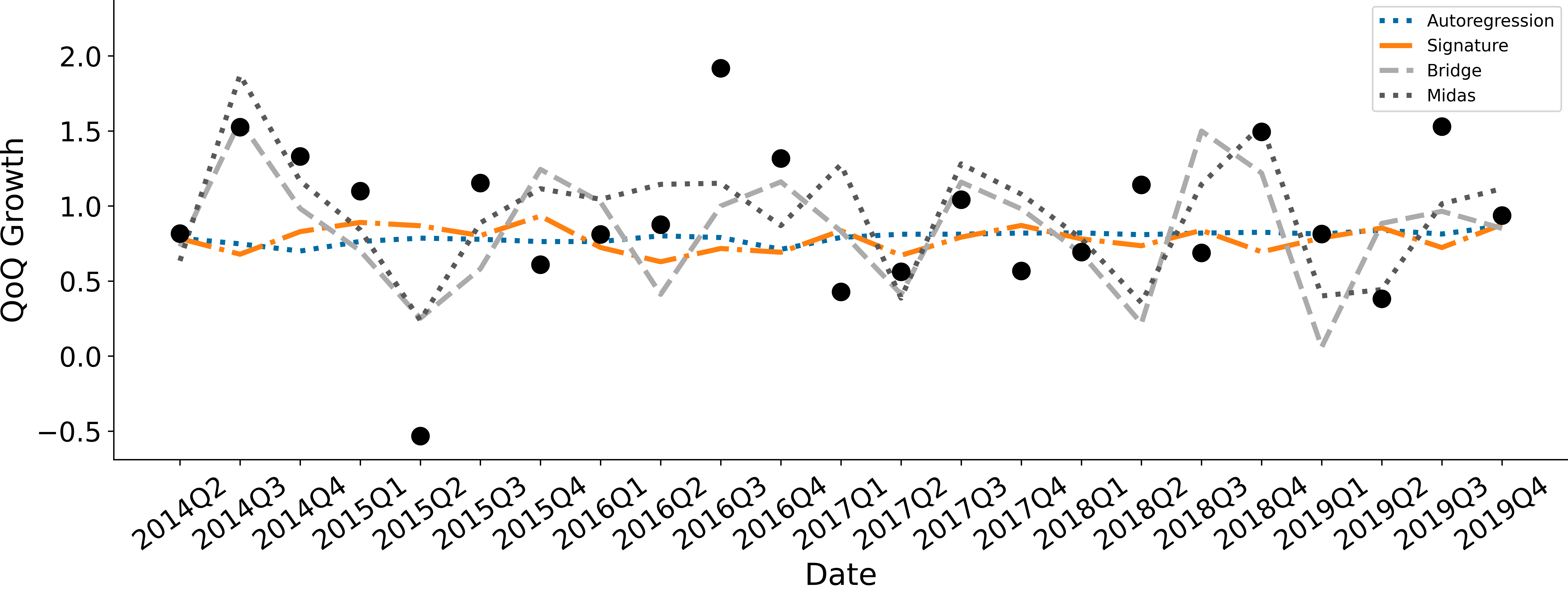
Figure 2: Nowcast model errors at horizon t+15 days
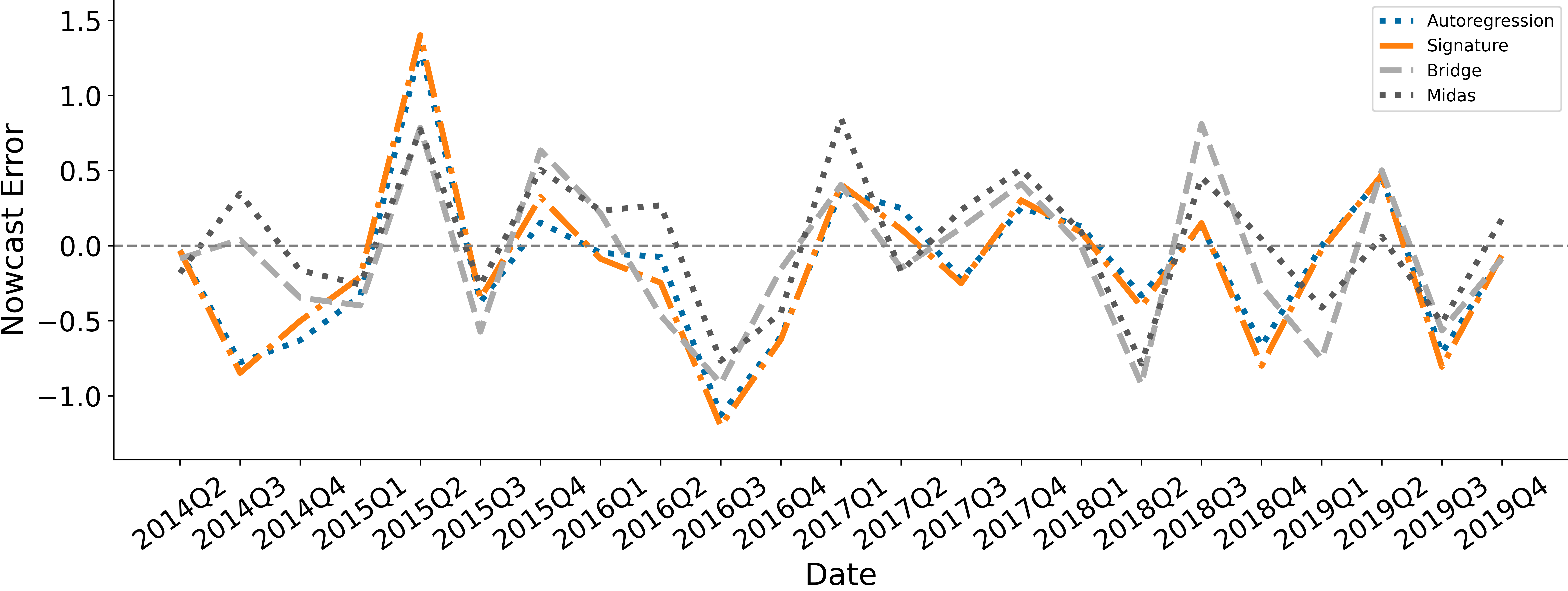
Table 2 Nowcast evaluation statistics
| t+0 days | t+15 days | t+45 days | |
| RMSE | |||
| AR(1) | 0.523 | 0.523 | 0.523 |
| Bridge | 0.451 | 0.505 | 0.553 |
| MIDAS | 0.371 | 0.440 | 0.404 |
| Signature | 0.489 | 0.558 | 0.556 |
| MAE | |||
| AR(1) | 0.395 | 0.395 | 0.395 |
| Bridge | 0.352 | 0.418 | 0.428 |
| MIDAS | 0.293 | 0.371 | 0.334 |
| Signature | 0.369 | 0.422 | 0.415 |
Figure 3: RMSE values for nowcasts across nowcast horizons
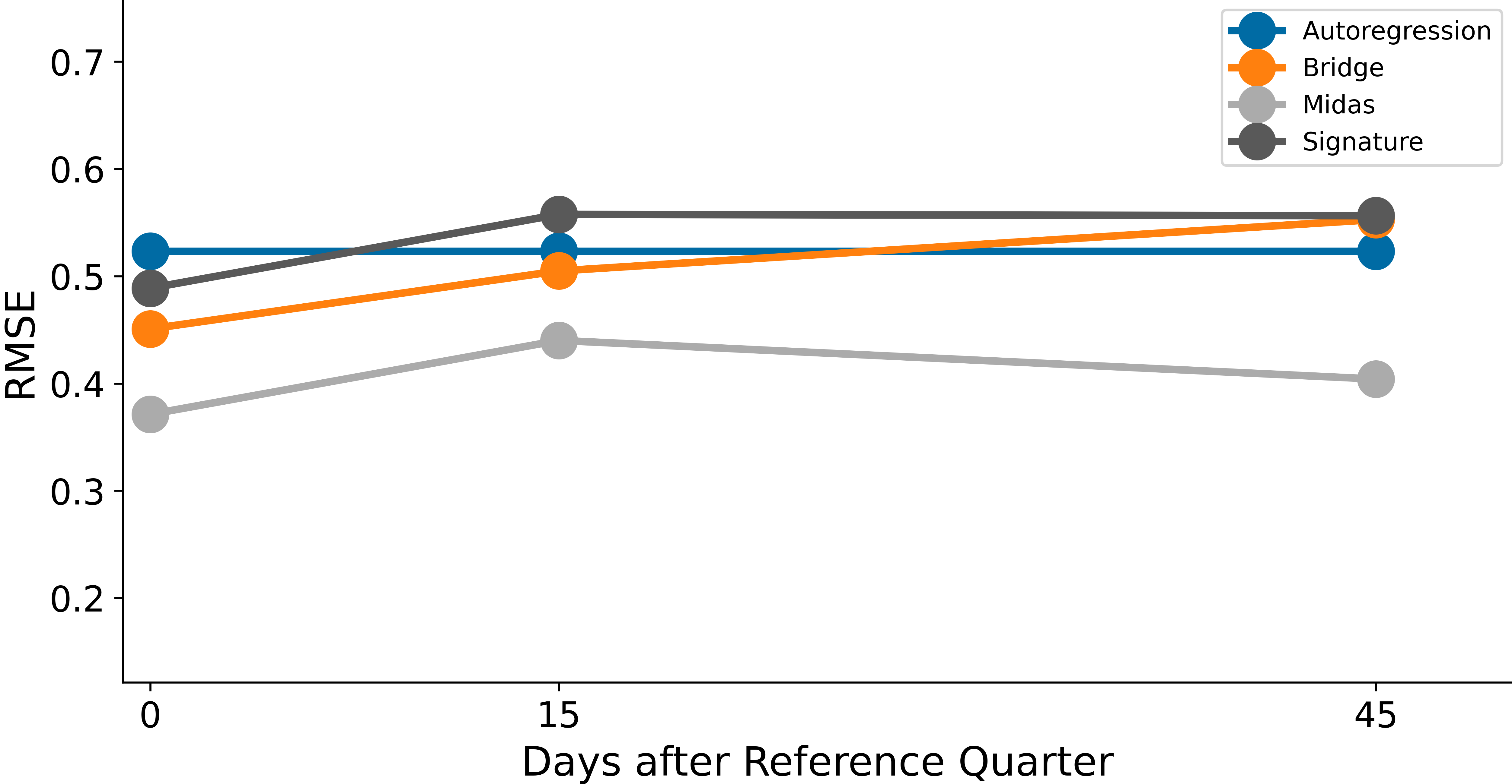
Figure 4: MAE values for nowcasts across nowcast horizons
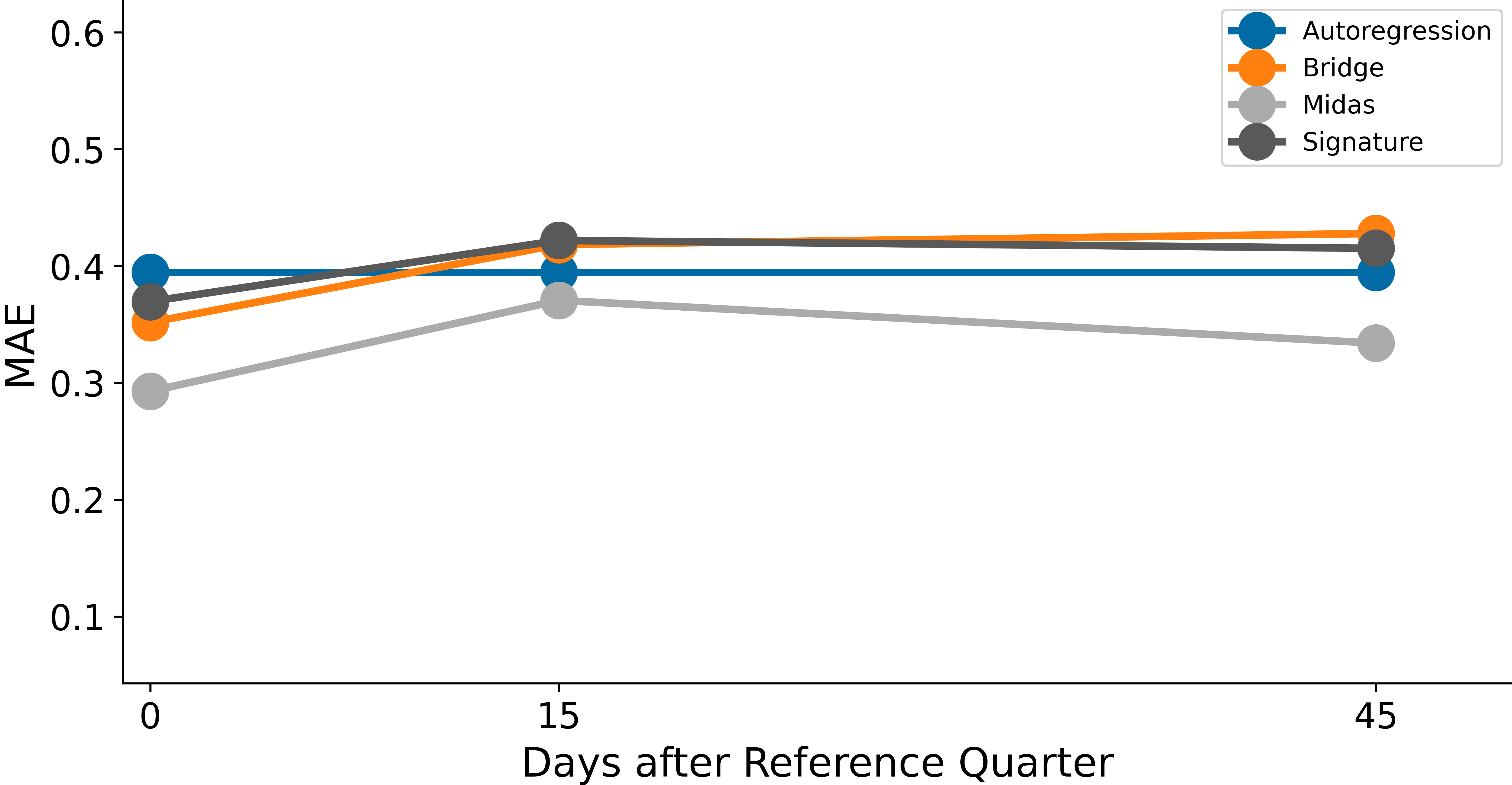
Figure 5: In-sample adjusted-R2 and absolute nowcast errors at horizon t+15 days for the bridge method
Selected subset of indicators
Using results from the bridge method, we look at how often individual indicators are selected, and which groups of indicators are chosen together under the shrinkage methods in the Variables section.
As described in the Recursive nowcasts section, we recursively estimate the nowcast model so there can be a different set of indicators selected at each quarter and each nowcast horizon. Since we find that both LASSO and Elastic Net, each used in conjunction with random forests, give similar results, we report the results we obtain using Elastic Net with the penalty ratio set to equally blend the L1 and L2 penalties. The results presented in this subsection are derived from bridge method, but as explained in the Variables selection section, the same set of selected indicators are also used to produce MIDAS nowcasts.
Figure 6 shows the frequency of individual variables being chosen by the combination of random forest and Elastic Net and used for income nowcasts at different horizons. Table 3 shows the most frequently selected groups of indicators. In all cases, models will include a constant.
The top five indicators chosen by Elastic Net for bridge nowcasts are Average Weekly Earnings (AWE), Index of Services (IOS), Retail Sales Index (RSI), House Price Index (HPI) and Manufacturing Production (MPROD). AWE, IOS, and RSI are chosen in over half of the models across each horizon. It is not surprising to see that these top five indicators are also included frequently in the top five subsets of chosen indicators, as shown in Table 3. Overall, the findings from our variable selection exercise shows that information about weekly household earnings, services and manufacturing output, retail sales, and house prices are the most useful in explaining changes in household income.
We observe that while some indicators are often being chosen as components of the subsets, the actual subset that is chosen by the shrinkage method varies in each recursive estimation. If relationships between the target variable and the indicators are stable, we expect to see the same set of indicators to be constantly chosen in the recursive estimation. The fact that we observe such variation in the subset of indicators implies that the explanatory power of the indicators varies across time. Moreover, we find that the adjusted R2 from the bridge method averages 0.44.
These findings provide some potential reasons as to why we do not observe an appealing empirical performance of the nowcasts produced. Firstly, the indicators we consider are not particularly strong in nowcasting household income; secondly, the usefulness of indicators change over time, so the variables that are selected based on in-sample performance may not be useful in nowcasting household income out-of-sample. The uncertainty of the usefulness of indicator variables across time may make prediction of household income challenging.
Figure 6: Proportion of quarters in the evaluation sample that a variable is selected across all horizons
Table 3: Number of times the top five subsets of indicators chosen by Elastic Net are selected across quarters in the evaluation sample
| Variable Subset | t+0 | t+15 | t+45 | Total |
| AWE, IOS, MPROD, RSI | 2 | 3 | 3 | 8 |
| AWE, CCI, IOS, NCC, RSI | 2 | 2 | 2 | 6 |
| AWE, HPI, IOS, RSI | 2 | 1 | 3 | 6 |
| AWE, HPI, IOS, SEER | 2 | 2 | 2 | 6 |
| AWE, IOS, MPROD | 2 | 1 | 2 | 5 |
4. Conclusion
In this technical report, we develop nowcasts of UK household income using data that covers information about different parts of the economy and a selection of time series methods.
This report is part of a programme of work that the Office for National Statistics (ONS) has been doing with the Alan Turing Institute to explore the usefulness of various economic nowcasting methods, particularly the signature method. Other outputs from our work may also be of interest. A paper released contains more information on the how the signature method compares mathematically against other methods and details its empirical performance in other settings, including nowcasting US gross domestic product (GDP). There is also a PYTHON code repo, which enables others to apply the signature method to generate nowcasts for other variables of interest.
We find that nowcasting UK household income is challenging. We find that the mixed-data sampling (MIDAS) method offers a slight improvement over an autoregressive baseline. One potential advantage is it manages to capture some of the movement in the household income realisations, whereas the autoregressive model is a broadly constant nowcast, which may be less useful during periods of rapid change in household income.
Other methods, including the signature method, produce similar results to the autoregressive baseline and there is limited improvement as data on more indicators become available. The signature regression method has had a stronger relative performance in other contexts we have studied as part of this programme of work (see paper).
Although we find that the variables in use do not contain strong information for predicting household income, we do find a pattern of core variables that show up frequently throughout the evaluation period. The explanatory variables that seem to have the most power are Average Weekly Earnings (AWE), Index of Services (IOS), Retail Sales Index (RSI), House Price Index (HPI), and Manufacturing Production (MPROD). Of these, AWE, IOS and RSI are chosen in over half of the models across each of the horizons. However, the combinations of the subset of indicators used to produce nowcasts are changing overtime.
This research has been useful for the household income team and the ONS, as they seek the best methods for the development of their estimates so policymakers can gain the best early indications about the state of the economy.
5. Author affiliations
Samuel N. Cohen also affiliates to the University of Oxford
Silvia Lui also affiliates to the Economic Statistics Centre of Excellence
Giulia Mantoan also affiliates to the Office for National Statistics,
Lars Nesheim also affiliates to the University College London
Aureo de Paula also affiliates to the University College London
Lingyi Yang also affiliates to the Office for National Statistics and the University of Oxford.
6. Disclaimers
The views expressed are those of the authors and may not reflect the views of the Office for National Statistics or the wider UK government.
Any views expressed are solely those of the author(s) and so cannot be taken to represent those of the Bank of England or to state Bank of England policy. This paper should therefore not be reported as representing the views of the Bank of England or members of the Monetary Policy Committee, Financial Policy Committee or Prudential Regulation Committee.